K K ij ij ijk 2 = r ! K ij "#$% 1 ! r ! ln( h r ij 1 ) () h ij 1 () + + h ij 3 ()

OS1203

Copyright©社団法人 日本機械学会

1. Introduction

Dissimilar material joints have singularities created by discontinuities in material properties across an interface. For this reason, it is difficult to predict an accurate stress by using a conventional FEM. There are some special elements or methods developed for solving this problem. An enriched finite element method developed by Benzley⁽¹⁾ is one method that do not need to divide into very small meshes around the singular point and can directly compute the intensity of singularity, while the conventional FEM is hard to separate the intensity of singularities in case of multi-singularities.

In the present study, the singular stress field in three-material joints with power-logarithmic singularities is analyzed by an enriched finite element method. Eigenvalue and eigenvector analyses are applied to calculate the order of stress singularities and the asymptotic displacement fields on the enriched elements. The method is modified by changing a mesh type from 4-node to 8-node elements. Enriched

element size and area are varied to study its convergence and to find a suitable element for each case. In addition, the joint models with various lengths are investigated to study the influence of geometries on the singular stress field.

2. Analytical formula

2D singular stress field around the singular point with power-logarithmic stress singularities can be described by

!_ij=Kij1r^!"h_ij1(#)+

Kij2r^!""#!ln(r)h_ij1(#)+h_ij3(#)$% (1) where r is the radial distance from the singular point, λis the order of stress singularity, Kijkand h_ijk(θ^{); (i, j}

= r or θ, k = 1, 2), are the intensity of singularities and angular functions, respectively.

2D enriched element equations were developed by Benzley⁽¹⁾ to solve an intensity in stress and displacement fields at two-dimensional singular point.

In this method, three different elements; enriched, transition and standard elements, are used. (See Fig.1)

対数特異性を有する三相接合体のエンリッチ有限要素法を用いた特 異応力場の強さの解析

（形状寸法の影響）

Analysis of intensity of singularity for three-materials joints with power-logarithmic singularities using an enriched finite element

method

（ Discussion on an influence of the geometry）

Chonlada LUANGARPA

and Hideo KOGUCHI

*1 Graduate school of Nagaoka University of Technology 1603-1 Kamitomioka, Niigata

*2 Nagaoka University of Technology 1603-1 Kamitomioka, Niigata

In the present study, the enriched finite element method is applied to compute the intensity of singularity for three-material joints with power-logarithmic singularities. The method is modified by using a higher order polynomial function, i.e., changing an element type from linear to quadratic element. Different sizes of the enriched region and mesh refinement technique are used to study its convergence. Furthermore, the models with various lengths are investigated to study an influence of geometry on the singular stress field.

Key Words : Stress singularity, Enriched finite element method, Power-logarithmic singularity

*1正員，長岡技術科学大学大学院（〒940-2188 長岡市上富岡町 1603-1）

*2正員，長岡技術科学大学 工学部．

E-mail: [email protected]

The displacement assumption for the enriched element is of form

(2)

In eq.(2), u1 and u2 represent the displacements of a point within the element in the x- and y- directions, respectively. Q_k1 and Q_k3 are the asymptotic displacement fields. u^kn , Q_kn1 and Q_kn3 are the values of u_k , Q_k1(r,!) and Q_k3(r,!) evaluated at node n, m is the number of node in an element and gn

is the shape function in a standard finite element.

For transition elements (type B element), they are needed to join enriched elements to standard elements in a finite element model. The displacement field in a transition element is given by the relationship

(3)

where R(ξ^,η) is a ‘zeroing’ function, equals to 1 along

‘enrich’ boundaries and equals to 0 along ‘standard’

boundaries.

3. Numerical analysis 3・1 The model for analysis

The model for analysis is the three-material joint fixed on the bottom side and subjected to shear loading (τ0 = 1 MPa) on the top surface, as shown in Fig. 2.

Plane strain condition is considered. Material properties are shown in Table 1.

At first, the model that is fixed its thickness, h, at 10 mm and its length, L, at 60 mm is chosen to study the influence of mesh refinement and the enriched area size. And then, in order to study a relationship between the intensity of singularity and model’s size, the

Fig. 1 Element models for Enriched Analysis

models that are fixed its thickness (h= 10 mm) and varied its length (L) from 60 to 300 mm are analyzed.

3・2 Eigenvalue analysis

Eigenvalue analysis by FEM is used to find the asymptotic displacement fields in the enriched element.

The eigen equation can be expressed as:

(4) where [A], [B] and [C] are matrices compose of Young’s modulus and Poisson’s ratio, p = 1-λ and {u} is the eigenvector of displacement.

The results from eigen analysis show that there are 2 real-singularities which the orders of stress singularity (λ1 = 0.3474 and λ2= 0.3466) are very close together.

At the next step, eigenvector analysis is applied to evaluate the angular displacements, which are then converted to the angular functions; hij1(θ) and hij3(θ) in eq.(1), for the stress and displacement relationships shown in Fig. 3.

Fig. 2 Analytical model and boundary condition Table 1 Material properties

Young’s modulus (GPa)(GPa)

Poisson’s ratio Material 1

(M1)

160.0 0.3

Material 2 (M2)

4.0 0.3

Material 3 (M3)

16.123 0.3

Fig. 3 Angular functions; hij1 and hij3 respectively

(p²[A]+p[B]+[C]){u}=0

1.0 0.5 0.0 -0.5 hij1

-180 -90 0 90 180

!  h_!!1

h_r!1

20 15 10 5 0 -5 -10 hij3

-180 -90 0 90 180

! h_!!3 h_r!3

u_k= g_n

n=1

!

n=1

!

K!!2 "ln(r)Q_k1+Q_k3" g_n

n=1

!

#

$% &

'(

u_k= g_n

n=1

!

n=1

!

K##2["ln(r)Q_k1+Q_k3" g_n

n=1

!

3・3 Enriched FEM

The element model around the singular point is shown in Fig. 1. 8-node element is used. To study the influence of mesh refinement and the enriched area size on the result convergence, the size of enriched elements, b, is varied from 0.05 to 1.0 mm and the enriched area, a, is varied from 0.5 to 4.0 mm (applied to the model with its fixed length, L, at 60 mm).

The results of the intensity of singularities (K!!1and K!!2) with various enriched element sizes and various enriched areas are shown in Figs. 4-5. In this study, the results are compared with conventional FEM’s results (analyzed by Marc program) which determine the intensity of singularities following Munz and Yang⁽²⁾’s fitting technique (K_θθ1 = 1.609 and K_θθ2 = 0.244). As can be seen on these figures, the intensity of singularities converges to the results in the conventional FEM when the element size is smaller.

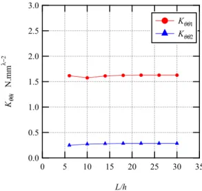
Next, in order to investigate a relationship between the intensity of singularity and model’s size, the model with enriched element size, b, = 0.1 mm and the enriched region size, a, of 0.5x0.5 mm² are employed.

The intensities of singularity, K_θθ1 and K_θθ2, with various lengths (L = 60 - 300 mm) for fixed thickness (h = 10 mm) are shown in Fig. 6. These results show that the intensities of singularity, both K_θθ1 and K_θθ2, are constant even if the length of the model increases.

4. Conclusions

The results obtained applying the enriched FEM on power-logarithmic singularities model were agreed with those using the conventional FEM. The accuracy of the results can be improved by using the smaller size of the enriched elements. Finally, the results for various model lengths show that the intensities of singularity are constant even if the length of the model increases.

References

(1) Benzley, S.E., Int. J. Numerical Methods in Engineering, 8, 537-545 (1974)

(2) D. Munz and Y.Y. Yang, Int. J. Fracture, 60, 169-177 (1993)

(3) Pageau S.S., Bigger S.B., Int. J. Numerical Methods in Engineering, 40, 2693-2713 (1997)

(4) Koguchi, H and Luangarpa, C., Journal of Solid Mechanics and Materials Engineering, Vol. 2, 319-332, (2008)

Fig. 4 The 1^st intensity of singularity, K_θθ1, against enriched area

Fig. 5 The 2^nd intensity of singularity, K_θθ2, against enriched area

Fig. 6 The intensities of singularity, K_θθi, against L/h 2.0

1.9 1.8 1.7 1.6 1.5 K!!1 N.mm"-2

5 4 3 2 1 0

a mm (Enriched area = a²) b = 0.05 mm b = 0.1 mm b = 0.5 mm b = 1.0 mm Marc

0.30 0.28 0.26 0.24 0.22 0.20 K!!2 N.mm"-2

5 4 3 2 1 0

a mm (Enriched area = a²) b = 0.05 mm b = 0.1 mm b = 0.5 mm b = 1.0 mm Marc

3.0 2.5 2.0 1.5 1.0 0.5 0.0 K!!i N.mm"#2

35 30 25 20 15 10 5 0

L/h

 K_!!1  K_!!2