Application of an enriched FEM to 2D-dissimilar material joints (Application in 2-real singularities model)

(1)

1. Introduction

Dissimilar material joints have singularities created by discontinuities in material properties across an interface. For this reason, it is difficult to predict accurate stress by using conventional FEM. There are some special elements or methods developed for solving this problem. An enriched finite element method developed by Benzley⁽¹⁾ is one method that do not need to divide meshes around the singular point to be very small meshes and can directly compute the intensity of singularity while conventional FEM hard to separate the intensity of singularities in case of multi singularities.

In the present study, the singular stress field in three-material joints with 2-real singularities is analyzed by an enriched finite element method. An eigenvalue and eigenvector analysis is applied to calculate the order of stress singularities and the asymptotic displacement fields on the enriched elements. This study is focused on the effect of changing element shape function (changed from 4-node element to 8-node element) on the accuracy of the results. Furthermore, enriched element size and area are varied to study its convergence and to find a suitable element for each case.

2. Analytical formula

2-D singular stress field around the singular point with two stress singularities can be described by !_ij =K₁r^"#¹f_ij1($)+K₂r^"#²f_ij2($) (1) where r is the radial distance from the singular point,

λ_k, Kk and fijk(θ); (k = 1,2), are the orders of the stress singularity, stress intensity factors and angular functions, respectively.

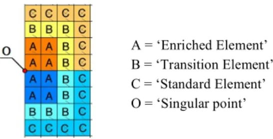
2-D enriched element equations were developed by Benzley⁽¹⁾ to solve an intensity in stress and displacement for two-dimensional singular point. In this method, three different elements; enriched, transition and standard elements, are used. (See Fig.1)

Fig. 1 Element models for Enriched Analysis The displacement assumption for the enriched element is of form

(2)

In eq.(2), u₁ and u₂ represent the displacements of a point within the element in the x- and y- directions, respectively. Q_k1 and Q_k2 are the intensities of singular terms (unknown coefficients) for λ1 and λ2, respectively. ukn, Q_kn1 and Q_kn2are the values of u_k , Q_k1(r,!)^and Q_k2(r,!) evaluated at node n, m is the number of node in an element and g_n is the standard finite element shape function.

二次元接合体に対するエンリッチ有限要素法の適用

（２つの特異性のオーダがある場合）

Application of an enriched FEM to 2D-dissimilar material joints (Application in 2-real singularities model)

Chonlada LUANGARPA

^*1

and Hideo KOGUCHI

^*2

*¹ Graduate school of Nagaoka University of Technology 1603-1Kamitomioka, Niigata

*² Nagaoka University of Technology 1603-1Kamitomioka, Niigata

In this study, the enriched finite element method is applied to compute the intensity of singularity for dissimilar material joints with 2-real singularities. Different mesh types and different size of the enriched region are applied to improve an accuracy of the results. It is shown that the results from applied the enriched FEM to the 3-material junction is agreed with those using a conventional FEM. In addition, numerical error is reduced by changing mesh types from linear to quadratic elements.

Key Words : Stress singularity, Enriched finite element method, Intensity of singularity

A = ‘Enriched Element’

B = ‘Transition Element’

C = ‘Standard Element’

O = ‘Singular point’

u_k = g_n

n=1

!

m ^u^kn⁺^K""1(Q_k1# g_n

n=1

!

m ^Q^kn1⁾

+K_""₂(Q_k2# g_n

n=1

!

m ^Q^kn2⁾

(2)

For transition elements (type B element), they are needed to join enriched elements to standard elements in a finite element model. The displacement field in a transition element is given by the relationship

u_k = g_n

n=1

!

m ^u^kn⁺R(",#){K_$$1(Q_k1% g_n

n=1

!

m ^Q^kn1⁾

+K_$$2(Q_k2% g_n

n=1

!

m ^Q^kn2^)} ⁽³⁾

where R(ξ^,η) is a ‘zeroing’ function, equals to 1 along

‘enrich’ boundaries and equals to 0 along ‘standard’

boundaries.

For finding the asymptotic displacement fields on enriched element, an eigen value analysis by FEM is separately carried out. By using eigen analysis method, the order of the stress singularity λ and the angular variation of the displacement fields can be determined in polar coordinates (ur, uθ). Then, the function Qij (i, j=1, 2) from converted polar coordinates data to Cartesian coordinates may be written as

Q_1j =r^!^j(u_rj(") cos(")#u_"j(")sin(")) /E

Q₂_j =r^!^j(u_rj(")sin(")+u_"_j(") cos(")) /E

(4)

where E is Young’s modulus of material 1.

3. Numericalanalysis

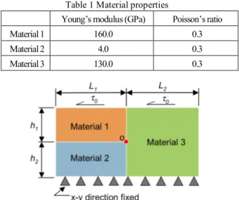
3-1 The model for analysis The model for analysis is shown in Fig 2. It is the three-material model fixed on the bottom side and applied shear stress on the top.

For this analysis, the height of material 1 and material 2 are fixed at 20 mm (h₁ = h₂ =20 mm). The model length L1 and L2 are equally at 60 mm and shear loading on the top surface is 1 MPa. Material properties are showed in Table 1.

3-2 Eigenvalue analysis Eigen analysis is used to find displacement fields in the enriched element. The eigen equation can be expressed as:

(p²[A]+p[B]+[C]){u}=0 (5) where [A], [B] and [C] are matrices compose of Young’s modulus and Poisson’s ratio, p = 1-λ and {u} is the eigenvector of displacement.

The orders of stress singularity (λ1 and λ2) from eigenvalue analysis are 0.4289 and 0.1027. The angular variations of displacement (u_rj and u_θj in eq.(4)) are analyzed by eigenvector analysis. Figure 3 shows the displacement profile for λ1 and λ2, respectively. Angular functions (f_ij1(θ) and f_ij2(θ)ⁱⁿ eq.(1)), those are evaluated by converting displacements to stresses, are shown in Fig. 4.

Table 1 Material properties

Young’s modulus (GPa) Poisson’s ratio Material 1

(M1)

160.0 0.3

Material 2 (M2)

4.0 0.3

Material 3 (M3)

130.0 0.3

Fig. 2 Analytical model and boundary condition

-0.08 -0.04 0.00 0.04 0.08

Displacement

-180 -90 0 90 180

θ

ur1

u_!1

Fig. 3 Displacement fields for λ₁ and λ₂ respectively

-1.0 -0.5 0.0 0.5 1.0

Angular function

-180 -90 0 90 180

θ

f_{!! 1} f_{r! 1}

Fig. 4 Angular functions for λ₁ and λ₂ respectively 3-3 Enriched FEM On this analysis, 8-node element is used to improve an accuracy of analysis.

The element model around the singular point is shown in Fig. 5. To study the influence of mesh refinement and the enriched area size on the result convergence, the size of enriched elements (b) is changed from 0.1 to 5.0 mm. and the enriched area (a) is varied from 0.1 to 6.0 mm.

Fig. 5 Element model around the singular point

0.30

0.20

0.10

0.00

Displacement

-180 -90 0 90 180

θ

u_r2

u_{! 2}

-1.0 -0.5 0.0 0.5 1.0

Angular function

-180 -90 0 90 180

θ f_{!! 2} f_r_{! 2}

(3)

The results of the intensity of singularities (K_θθ1 and K_θθ2) with various enriched element sizes and various enriched areas are shown in Figs. 6-9. In this study, the results are compared with conventional FEM’s results (analyzed by Mentat program) which determine the intensity of singularities followed Munz and Yang⁽²⁾’s fitting technique. Figures 6 and 8 show the results of K_θθ1 and K_θθ2 by using 4-node element models. As can be seen on these figures, the intensity of singularities converges to the result in Mentat when the element size is smaller. After changing to 8-node elements, as shown in Figs. 7 and 9, the results are going to the same direction as 4-node element’s results, but convergence rate is much better. In addition, by using 8-node elements, the intensity of singularities is little influenced from enriched area’s size.

4. Conclusions

The results obtained applying the enriched FEM on 2-real singularities model are agreed with those using conventional FEM. The accuracy of the results can be improved by changing the element shape function from 1-order to 2-order polynomial functions. For modeling selection, an enriched element size should be smaller than a singular area.

5. References

(1) Benzley, S.E., Int. J. Numerical Methods in Engineering, 8, 537-545 (1974)

(2) D. Munz and Y.Y. Yang, Int. J. Fracture, 60, 169-177 (1993)

(3) Pageau S.S., Bigger S.B., Int. J. Numerical Methods in Engineering, 40, 2693-2713 (1997)

(4) Koguchi, H and Luangarpa, C., Journal of Solid Mechanics and Materials Engineering, Vol. 2, 319-332, (2008).

4.4 4.2 4.0 3.8 3.6 3.4 K!!1 (N.mm"1-2 )

6 5 4 3 2 1 0

a mm. (Enriched area = a²) b = 0.1 mm.

b = 0.5 mm.

b = 1.0 mm.

b = 2.0 mm.

b = 5.0 mm.

Mentat

Fig. 6 The 1-intensity of singularity (K_θθ₁) against enriched area (4-node element models)

Fig. 7 The intensity of singularity, K_θθ₁, against enriched area (8-node element models)

-4.0 -3.8 -3.6 -3.4 -3.2 -3.0

K!!2 (N.mm"2-2 )

6 5 4 3 2 1 0

b = 0.5 mm.

b = 1.0 mm.

b = 2.0 mm.

b = 5.0 mm.

Mentat

Fig. 8 The 2-intensity of singularity (K_θθ2) against enriched area (4-node element models)

-4.0 -3.8 -3.6 -3.4 -3.2 -3.0

K!!2 (N.mm"2-2 )

6 5 4 3 2 1 0

b = 0.5 mm.

b = 1.0 mm.

b = 2.0 mm.

b = 5.0 mm.

Mentat

Fig. 9 The 2-intensity of singularity (K_θθ₂) against enriched area (8-node element models)

4.4

4.2

4.0

3.8

3.6

3.4 K!!1 (N.mm"1-2 )

6 5 4 3 2 1 0

b = 0.5 mm.

b = 1.0 mm.

b = 2.0 mm.

b = 5.0 mm.

Mentat