Q Q %&'( #$%&'( K K = K r h () + K r " ln( r ) h () + h () u = g u + K Q " g Q + ! ! #$%&'( K " ln( r ) Q + Q " g ( " ln( r ) Q + Q ) !

JSME-CMD International Computational Mechanics Symposium 2012 in Kobe (JSME-CMD ICMS2012)

1

Evaluation of intensity of singularity for three-materials joints with power-logarithmic

singularities using an enriched finite element method*

Chonlada LUANGARPA**and Hideo KOGUCHI***

**Graduate School of Nagaoka University of Technology 1603-1 Kamitomioka, Niigata, Japan

E-mail:[email protected]

*** Nagaoka University of Technology 1603-1 Kamitomioka, Niigata, Japan

In this study, the enriched FEM is applied to compute intensity of singularity for three-material joints with power-logarithmic singularities. The models with various lengths and thicknesses are investigated to study an influence of geometry on the singular stress field.

Key words: Stress Singularity, Enriched Finite Element Method, Intensity of Singularity, Power-logarithmic Singularity

1. Introduction

In the present study, the singular stress field in three-material joints with power-logarithmic singularities is analyzed by an enriched finite element method. This method was firstly developed by Benzley⁽¹⁾ for cracks in 2D elastic solids. An eigenvalue and eigenvector analysis (Pageau and Bigger⁽²⁾) are applied to calculate the order of stress singularities and the asymptotic displacement fields on the enriched elements. The joint models with various lengths and thicknesses are investigated to study an influence of geometry on the singular stress field.

2. Analytical formula

2D singular stress field around the singular point with power-logarithmic stress singularities can be described by

!_ij =Kij1r^"#h_ij1($)+Kij2r^"#%&"ln(r)h_ij1($)+h_ij3($)'( (1)

where r is the radial distance from the singular point, λ1, λ2 are the order of stress singularity. Kij1, Kij2 and h_ij1(θ^{), h}ij3(θ); i, j = r or θ, are the intensities of singularity and angular functions, respectively.

In this method, 3 types of element; enriched, transition and standard elements, are employed. The displacement assumption in an enriched element is of form

u_k = g_n

n=1

!

n=1

!

#

$% &

'(+ Kij2 "ln(r)Q_k1+Q_k3" g_n

n=1

!

#

$% &

'(

(2)

In Eq. (2), u1 and u2 represent the displacements of a point within the element in the x and y directions, respectively. Q_k1and Q_k3 are the asymptotic displacement fields related

JSME-CMD International

Computational Mechanics Symposium 2012 in Kobe (JSME-CMD ICMS2012)

2 to the angular functions h_ij1 and h_ij3 in Eq. (1), respectively. u^kn, Q_kn1 and Q_kn3are the values of uk , Q_k1(r,!) and Q_k3(r,!) evaluated at node n.

The displacement field in a transition element is given by the relationship

u_k = g_n

n=1

!

n=1

!

Kij2[$ln(r)Q_k1+Q_k3$ g_n

n=1

!

where R(ξ^,η) is set a ‘zeroing’ function, equals 1 along ‘enrich’ boundaries and equals 0 along ‘standard’ boundaries.

3. Numerical analysis

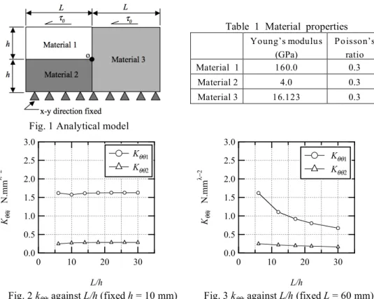
The model for analysis is shown in Fig 1. It is the three-material model fixed on the bottom side and applied shear stress (τ0 = 1 MPa) on the top. Material properties are shown in Table 1. The intensities of singularity with various lengths (L = 60-300 mm) for fixed thickness (h = 10 mm) are shown in Fig. 2. In the same way, the intensities of singularity with various thicknesses (h = 2-10 mm) for fixed length (L = 60 mm) are shown in Fig. 3.

4. Conclusion

The enriched FEM was developed for calculating the intensity of singularity of power-logarithmic singularities. The results for various model lengths and thicknesses show that the intensities of singularity are constant with increasing of lengths but the intensities of singularity decrease with decreasing of thicknesses.

References

(1) Benzley, S.E., Representation of singularities with isoparametric finite elements, International Journal of Numerical Methods in Engineering, Vol. 8, (1974), pp. 537-545.

(2) Pageau, S.S., Biggers, S.B., Enrichedment of finite elements with numerical solutions for singular stress fields, International Journal of Numerical Methods in Engineering, Vol. 40, (1997), pp. 2693-2713.

Table 1 Material properties Young’s modulus 

(GPa)

Poisson’s ratio Material 1

(M1)

160.0 0.3

Material 2 (M2)

4.0 0.3

Material 3 (M3)

16.123 0.3

Fig. 1 Analytical model

Fig. 2 k_θθι against L/h (fixed h = 10 mm) Fig. 3 k_θθι against L/h (fixed L = 60 mm) 3.0

2.5 2.0 1.5 1.0 0.5 0.0 K!!i N.mm"#2

30 20 10 0

L/h

 K_!!1  K_!!2 

3.0 2.5 2.0 1.5 1.0 0.5 0.0 K!!i N.mm"#2

30 20 10 0

L/h

  K_!!1   K_!!2