衝撃波の干渉を伴う

(1)

衝撃波の干渉を伴う

超音速遷移 / 乱流境界層に関する直接数値シミュレーションによる研究

戸倉裕介

電気通信大学情報理工学研究科博士（工学）の学位申請論文

2013 年 3 月

(2)

衝撃波の干渉を伴う

超音速遷移 / 乱流境界層に関する直接数値シミュレーションによる研究

博士論文審査委員会

大川富雄教授前川博教授

Matuttis Hans-Georg 准教授宮嵜武教授

山本誠教授

(3)

著作権所有者

戸倉裕介

2013 年 3 月

(4)

Yusuke TOKURA

Abstract

Physical phenomena associated with turbulent boundary layers and shock waves are commonly observed in aerospace applications and are important to the development of high-speed vehicles and propulsion systems. Unsteady shock wave/boundary layer interactions ( hereafter referred as SWBLI ) are of extreme relevance for aerospace application design, such as aircraft performance, structural fatigue, and air intake efficiency reduction due to boundary layer separation. The interaction of shock waves with turbulent boundary layers is the subject of extensive research for its relevance in transonic, supersonic and hypersonic flows. A fundamental understanding of the complex physical phenomena is important to improve engineering models and to attempt to control their detrimental effects.

Compressible flow linear stability analyses of supersonic flows with or without SWBLI have been principally led in the transition context. In low-disturbance environments, such as flight, boundary layer transition to turbulence generally occurs through the uninterrupted growth of linear instabilities. After the linear regime, nonlinear stages generated in a boundary layer leads to rapid breakdown downstream, the turbulent boundary layer develops on the surface of the flight obstacle that comprises high aerodynamic loads. The shock wave interacts with either laminar or turbulent boundary layers, which depends on its geometry in the aerospace application. The majority of SWBLI investigations are about the shock/turbulent boundary layer interaction. A very limited number of studies of shock wave/transitional boundary layer interaction have been reported.

In the present study, a spatial DNS of a supersonic flat plate boundary layer flow at Mach 2.0 with impinging shock wave is analyzed. Effects of both transition and boundary layer growth require the application of the fully spatial formulation in a DNS without extended temporal simplifying assumptions.

We consider the problem of a shock impinging upon a transitional boundary layer. Despite many experimental, theoretical and numerical studies in the past years, the nonlinear regime of transition in supersonic flat-plate boundary layer is still not thoroughly understood. In the shock impinging boundary layers, boundary layers are developing under adverse pressure gradient beneath the impinging shock. For strong interactions the flow separates and the wall pressure rise occurs well ahead of the nominal shock impinging. Although this stage of the boundary layer has been less studied, we consider that this type of SWBLI is appropriate to understand the complicating effects of bulk flow compression due to the shock that contributes significantly to turbulence amplification and the formation of large-scale structures. The numerical methods employed are based on ( yet perfectible ) mature approaches available ( 5th-order Dissipative Compact Schemes, 4th-order Runge-Kutta along with standard grid resolution for wall-bounded flows ) which leads to an appropriate numerical compromise. The comparison or evaluation of numerical tools is outside of the scope of our priority objective.

(5)

Chapter 1 provides a detailed survey of the studies that have been performed on the subject of shock/turbulent boundary layer interaction.

Chapter 2 describes the numerical simulation methodology and includes the description of spatial discretization and time integration techniques along with the method of generation of the artificial shock.

Chapter 3 deals with the direct simulation of transitional boundary layers with the impinging oblique shock which is strong enough to induce the separation of boundary layer. In this chapter, the shock system and interaction-region dynamics are described and the energy spectrum of wall pressure fluctuation in the interaction-region is analyzed to understand the low-frequency unsteadiness.

In Chapter 4, linear-stability theory ( LST ) is used to get a comprehensive picture of the selective growth of the wavenumbers. This LST predicts that oblique instability waves are strongly amplified throughout the interaction-region and can trigger the breakdown mechanism.

In Chapter 5, we discusses the three-dimensional structures around the interaction-region by means of specially evolving transitional boundary layer with the impinging oblique shock forced with a combination of unstable mode obtained from LST in Chapter 4. This simulation confirms that oblique instability waves can trigger the breakdown mechanism such as the mixture of structures in supersonic boundary layer and supersonic plane wake.

Chapter 6 presents a detailed statistical analysis of the results for the base flow simulations, i.e., the simulation of turbulent boundary layers without shocks. The base simulations are validated against other numerical and experimental results.

Chapter 7 provides some general conclusions and future perspectives.

(6)

直接数値シミュレーションによる研究

戸倉裕介概要

スペースプレーンに用いられるスクラム／ラムジェットエンジンや超音速機ターボジェットエンジンの空気取入口 ( インテーク ) において，インテーク内の高速流れの中に発生する衝撃波の挙動がエンジンの性能に重大な影響を与える．一方，SRB ( Solid Rocket Booster：固体補助ロケット ) を有するロケットなどでは，打ち上げの際に SRB から生じた衝撃波がロケット本体表面に発達した境界層に入射することによって，局所的な圧力上昇や空力加熱が引き起こされることが知られている．このように，超音速や極超音速で飛行する飛翔体などでは，飛翔体表面で発達する境界層と衝撃波との干渉が起こり，局所的な加熱や境界層剥離などが生じて飛翔体の飛行特性を著しく変化させる．さらに，衝撃波の低周波振動による航空機機体の疲労損傷なども重要な問題である．衝撃波/境界層干渉は航空宇宙工学において古くから注目されている未解明な基本的問題の一つであり、干渉機構の詳細が解明されることによる研究成果の波及効果は大きい．

衝撃波/境界層干渉の研究は大きく分けると圧縮ランプによるものと入射衝撃波発生機器によって衝撃波発生させるという二つのケース分けることができ，これまでの研究では，実験の容易さから前者のケースが多く行われてきた．一方，後者においては、これまでに行われてきた入射衝撃波発生機器による研究は，ほとんどが衝撃波/層流境界層干渉もしくは衝撃波/乱流境界層干渉のどちらかであり，インテーク内の高速流れは層流－乱流遷移状態が存在するにもかかわらず，

衝撃波と干渉する層流境界層の乱流遷移について調べた研究はこれまでのところほとんど行われていない．

このような背景のもと，本研究では主流マッハ数 2.0 における衝撃波と乱流遷移境界層の干渉を対象とし，剥離を伴う超音速境界層流れが持つ不安定性及びその結果から得られる不安定波の非線形発達に伴う乱流遷移構造ならびに乱流遷移とショックシステムとの関係を，圧縮性粘性線形解析および高解像度空間発展直接数値シミュレーション ( DNS ) を用いて研究した結果について報告する．

最初に，広い波数帯にエネルギーをもつ，一様等方的ランダム撹乱を比較的大きな振幅で流入した DNS を行うことで，剥離領域における撹乱の挙動について把握および剥離を伴う超音速境界層における乱流遷移の特徴について考察した．ここでは，比較的大きな撹乱を与えた場合であっても剥離を伴うような超音速境界層の乱流遷移においては，干渉領域で ( 1,1 )，( 0,2 ) といった斜行波対による遷移に関連する成分の成長率が上流の点よりも大きくなっていることを示し，

また，これらの不安定波の成長により干渉領域において特徴的な渦構造およびトポロジー構造が観測された．

線形安定性解析では，衝撃波を伴う超音速境界層に対する不安定撹乱を得るための線形安定性

(7)

認でき，三次元波ではその傾向が顕著に表れることを確認した．すなわち，剥離領域では斜行波による遷移が優勢であることが推測された．また，圧縮性粘性線形解析の結果と二次元衝撃波/境界層DNSの結果を比較することで，線形解析の有効性を議論し，さらに，剥離領域における不安定波の非定常構造に対する役割についても示した．

線形解析で得られた不安定モードは，三次元衝撃波/境界層 DNS によってその剥離領域における非線形発達を追い，干渉領域での乱流遷移構造および剥離泡内のトポロジー構造に対する二次元，三次元モードの役割を調べた．ここでは，干渉領域における三次元構造について示し，剥離

泡内のCenter構造が不安定波により下流へと押し流され，再付着領域に近づくとFocus構造へと

変化し，この変化により流れ場に強い変動が生成され乱流遷移が促進されていることが確認された．また，このFocus構造は，Perry & Chong ( 1986, 1987 ) によって明らかにされたU-Shaped

separation構造とよく類似しており，三次元不安定波とU-Shaped separationに深い関係性があるこ

とを示唆した．

本研究は衝撃波を伴うような流れについては現時点での先端的スキーム ( 5次精度散逸コンパクトスキーム，6次精度コンパクトスキーム，4段階4 次精度ルンゲクッタ ) および線形安定性解析を行い，衝撃波による剥離を伴う超音速境界層の乱流遷移構造を明らかにした．そして，剥離を伴う超音速境界層における不安定モードの非線形発達との関係を明らかにしたことにより，

依然未解明点の多い超音速境界層の遷移形態の理解に対し１つの指針を与える．

(8)

図目次

第1章

Fig. 1.2.1 The structure of a ramp flow without boundary layer separation. Adapted from Arnal & Délery

( 2004 )

･････ 3

Fig. 1.2.2 The structure of a ramp flow with boundary layer separation. Adapted from Arnal & Délery

( 2004 )

･････ 4

Fig. 1.2.3 The structure of impinging-reflecting shock without boundary layer separation. Adapted from

Arnal & Délery ( 2004 )

･････ 5

Fig. 1.2.4 Mean wall-pressure distribution for a SWBLI, demonstrating the influence of shock upstream of its inviscid origin. Adapted from Délery & Dussauge ( 2009 )

･････ 5

Fig. 1.2.5 The structure of impinging-reflecting shock with boundary layer separation. Adapted from Arnal

& Délery ( 2004 )

･････ 6

Fig. 1.2.6 Wall pressure distribution, in shock separated flow Adapted from Délery & Dussauge ( 2009 )

･････ 7

Fig. 1.3.1 Wall-pressure distribution for laminar separation for various model configurations and Reynolds number at M = 2.3. Adapted from Chapman et al. ( 1957 )

･････ 8

Fig. 1.3.2 Surface streak patterns for compression corner flows at Mach 2.9. Adapted from Settles et al.

( 1979 )

･････ 9

Fig. 1.3.3 Wall pressure time-histories. Adapted from Dolling & Or ( 1985 )

･････ 10

Fig. 1.3.4 ( a ) to ( c ) demonstrate the longitudinal Reynolds stress evolution along interaction region for 8°, 16°and 20°compression corner angle. Adapted from Smits & Muck ( 1987 )

･････ 10

Fig. 1.3.5 Probability density function of the muss-flux profile. Adapted from Selig et al. ( 1989 )

･････ 11

(11)

Fig. 1.3.6 Relationship between incoming boundary layer and separation shock foot unsteadiness. Adapted from Beresh et al. ( 2002 )

･････ 11

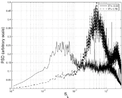
Fig. 1.3.7 Power spectral densities around the reflected shock with varying incident shock strength. Adapted from Dupont et al. ( 2006 )

･････ 12

Fig. 1.3.8 Schematic representation of the three-dimensional physical model. Adapted from Humble et al.

( 2009a )

･････ 13

Fig. 1.4.1 Sketch of the flow induced by a shock reflection with separation.

･････ 16

第2章

Fig. 2.6.1 Sketch of computational area and Cartesian coordinates.

･････ 32

第3章

Fig. 3.2.1 Comparison of skin friction coefficient with literatures.

･････ 38

Fig. 3.2.2 Comparison of simulation results with experimental data ( a ) skin-friction coefficient and ( b ) pressure distributions upstream/downstream of the impinging point. ( ximp: impinging point ).

･････ 38 Fig. 3.2.3 Mean Mach number contour.

･････ 39

Fig. 3.2.4 Reynolds stress contour. ( y×5 )

･････ 40

Fig. 3.2.5 ( a ) Skin-friction coefficient and ( b ) pressure distributions upstream/downstream of the impinging point: Comparison LES ( Teramoto ( 2005 ) ) and experimental measurement ( Hakkinen (1959) ). ( ξ = (x-xR)/(xR -xs); xR: mean reattachment point; xs: mean separation point ).

･････ 40

Fig. 3.2.6 Comparison of the mean streamwise velocitiy with Teramoto (red circle) and Hakkinen ( green rectangle ).

･････ 41

Fig. 3.2.7 Comparison of the Van Driest transformed mean streamwise velocity with Teramoto (left).

･････ 42

(12)

Fig. 3.2.8 Comparison of the R.M.S. velocity profiles with Teramoto (blue triangle), Prozzoli ( 2011, red circle ) and Schlatter ( 2011, green rectangle ).

･････ 42

Fig. 3.3.1 Mean density and pressure fields: ( top ) density field 0.6 <

 

_ < 1.3 ( 20 contour levels );

( bottom ) pressure field 0.17 < p p_ < 0.28 ( 20 contour levels ).

･････ 44

Fig. 3.3.2 Skin-friction coefficient and pressure distributions upstream/downstream of the impinging point.

･････ 45

Fig. 3.3.3 ( a ) ~ ( e ) PDFs of skin friction along a bubble at locations and ( f ) percentage of the mean flow forward ( red circle ) / reversed flow ( black circle ): ( a ) x = 40δ*0; ( b ) x = 80δ*0; ( c ) x = 120δ*0; ( d ) x = 140δ*0 and ( e ) x = 160δ*0.

･････ 46

Fig. 3.3.4 Turbulence intensity distributions: ( a ) 0.000 < u'rms / U_∞<0.027( 7 contour levels); ( b ) 0.000 <

v'rms / U_∞<0.005( 10 contour levels ) and ( c ) Reynolds stress -0.047 < u'v'/ U_∞<0.016( 10 contour levels).

･････ 47

Fig. 3.3.5 Anisotropy invariant maps of the Reynolds stress tensor in the boundary layer at various streamwise locations: The red line shows present case. The blue line shows without shock turbulent boundary layer (M = 2.3, Re_δ*0 = 4000) and the black line shows Lumley triangle. ( a ) the example of turbulent boundary layer case; ( b ) x = 80δ*0; ( c ) x = 10δ*0; ( d ) x = 160δ*0 and ( e ) x = 200δ*0.

･････ 48

Fig. 3.3.6 Distribution of mean streamwise velocity at various streamwise stations.

･････ 49

Fig. 3.3.7 Three-dimensional view of shock wave/turbulent boundary layer interaction, plotted by second invariant of velocity gradient tensor ( Q = 0.01 ) and reported by yellow; colored isosurfaces represent pressure.

･････ 50

Fig. 3.3.8 Isosurface plot of second invariant of velocity gradient tensor ( Q = 0.005 ): ( top ) top view and ( Bottom ) side view.

･････ 51

Fig. 3.3.9 Isosurface plot of low-speed streak ( u' = －0.1 ): ( top ) top view and ( bottom ) side view.

･････ 51

Fig. 3.3.10 Time sequence Isosurface plot of second invariant of velocity gradient tensor Q: ( a ) t = 230δ^*0 / U_∞;( b ) t = 250δ^*0 / U_∞; ( c ) t = 270δ^*0 / U_∞; ( d ) t = 290δ^*0 / U_∞ and ( e ) t = 300δ^*0 / U_∞.

･････ 52

Fig. 3.3.11 Time sequence of spanwise vorticity ωz at z = Lz/2: ( a ) t = 210δ^*0 / U_∞;( b ) t = 240δ^*0 / U_∞; ( c ) t = 260δ^*0 / U_∞; ( d ) t = 280δ^*0 / U_∞ and ( e ) t = 300δ^*0 / U_∞.

･････ 53

(13)

Fig. 3.3.12 Mean streamline: ( top ) at z/δ*0 = 12.0, x-y plane; ( bottom ) at y/δ*0 = 1.0, x-z plane; red broken line shows zero mean longitudinal velocity.

･････ 53

Fig. 3.3.13 Energy spectral density of the wall-pressure at various streamwise locations: ( a ) x = 80δ*0; ( b ) x = 110δ*0; ( c ) x = 120δ*0; ( d ) x = 140δ*0; ( e ) x = 160δ*0 and ( f ) x = 260δ*0.

･････ 54

Fig. 3.3.14 Development of the Fourier amplitudes in the downstream direction of selected modes.

･････ 55

第4章

Fig. 4.2.1 ( top ) instantaneous velocity field with streamline and ( bottom ) streamwise velocity at various streamwise points.

･････ 62

Fig. 4.2.2 Growth rate of two-dimensional wave at various streamwise stations.

･････ 63

Fig. 4.2.3 Growth rate of three-dimensional wave ( β = 0.3 ) at various streamwise stations.

･････ 63

Fig. 4.2.4 The most unstable value of instability wave growth rate ( red circle ) with wall pressure distribution ( solid line ).

･････ 65

Fig. 4.2.5 Contours of ωi obteined from LST: ( contour interval is 0.001 ) ( a ) x = 60δ*0; ( b ) x = 80δ*0; ( c ) x = 110δ*0 and ( d ) x = 130δ*0.

･････ 65

Fig. 4.2.6 Eigen functions for two-dimensional at various streamwise stations: black line: x = 60δ*0,; red line: x = 80δ*0; blue line: x = 110δ*0 and green line: x = 130δ*0.

･････ 66

Fig. 4.2.7 Eigen functions for two-dimensional at various streamwise stations: black line: x = 60δ*0,; red line: x = 80δ*0; blue line: x = 110δ*0 and green line: x = 130δ*0.

･････ 66

Fig. 4.2.8 Comparison between DNS and eigen function: black line and red line show DNS and eigen function respectively; solid line and broken line streamwise show velocity component and pressure component respectively.

･････ 67

Fig. 4.2.9 Instantaneous streamwise velocity fluctuation obtained from two-dimensional DNS: ( top ) ω = 0.09 case and ( bottom ) ω = 0.3 case.

････ 68

(14)

Fig. 4.2.10 Comparison of streamwise velocity R.M.S. value between ω = 0.09 case and ω = 0.3 case at various streamwise stations: black line and red line show ω = 0.09 case and ω = 0.3 case respectively.

･････ 68

Fig. 4.2.11 Instantaneous density gradient |∇ρ| obtained from two-dimensional DNS, ( top ) ω = 0.09 case and ( bottom ) ω = 0.3 case.

･････ 69

第5章

Fig. 5.1.1 The analysis of linear-stability theory ( M = 2.0, Re_δ*0 = 1000 ): ( a ) eigen function and ( b ) contours of growth rate ( with increment 0.0001 ).

･････ 72

Fig. 5.2.1 Mean density field 0.56 <  _ < 1.36 ( 22 contour levels )

･････ 72

Fig. 5.2.2 Skin-friction coefficient and pressure distributions upstream/downstream of the impinging point.

･････ 73

Fig. 5.2.3 Distribution of mean streamwise velocity at various streamwise stations.

･････ 74

Fig. 5.2.4 Time sequence isosurface plot of second invariant of velocity gradient tensor Q ( = 0.0002 ) at x-z plane: ( a ) t = 275δ^*0 / U_∞;( b ) t = 300δ^*0 / U_∞; ( c ) t = 325δ^*0 / U_∞; ( d ) t = 375δ^*0 / U_∞; ( e ) t = 400δ^*0 / U_∞; ( f ) t = 425δ^*0 / U_∞ and (g) t = 450δ^*0 / U_∞.

･････ 75

Fig. 5.2.5 Time sequence isosurface plot of second invariant of velocity gradient tensor Q ( = 0.0002 ) at x-y plane). (a) t = 275δ^*0 / U_∞,(b) t = 300δ^*0 / U_∞, (c) t = 325δ^*0 / U_∞, (d) t = 375δ^*0 / U_∞, (e) t = 400δ^*0 / U_∞, (f) t =425δ^*0 / U_∞ and (g) t = 450δ^*0 / U_∞.

･････ 76

Fig. 5.2.6 Time sequence of spanwise vorticity ωz at z /δ^*0 = 0: ( a ) t = 275δ^*0 / U_∞;( b ) t = 300δ^*0 / U_∞;( c ) t= 325δ^*0 / U_∞; ( d ) t = 375δ^*0 / U_∞; ( e ) t = 400/ U_∞; ( f ) t = 425δ^*0 / U_∞ and ( g ) t = 450δ^*0 / U_∞.

･････ 77

Fig. 5.2.7 Turbulence intensity distributions, ( a ) u'rms / U_∞, ( b ) v'rms / U_∞.

･････ 77

Fig. 5.2.8 Development of the Fourier amplitudes in the downstream direction of selected modes.

･････ 78

Fig. 5.2.9 Instantaneous velocity field ( velocity vectors ) and streamewise velocity ( color contour ), enclosed region in fig. 5.5: ( a ) x = 140δ*0; ( b ) x = 160δ*0; ( c ) x = 200δ*0 and ( d ) x = 220δ*0.

･････ 79

(15)

Fig. 5.2.10 ( a ) Instantaneous velocity field ( velocity vectors ) and streamewise velocity ( color contour ), ( b ) Average velocity field with u y( broken line, 0.3 < u y < 0.9, contour increment 0.1 ) and u z( solid line, -0.18 < u z< -0.04, 0.04 < u z< 0.018, contour increment 0.02 ),( c ) Average velocity field with R.M.S ( 0 < u'rms / U_∞ < 0.024, contour increment 0.004 ).

･････ 80 Fig. 5.3.1 (a) classification of critical points on the p–q chart, (b) degenerate critical points, or borderline

cases; case numbers refer to (a). Adapted from Perry and Chong ( 1987 )

･････ 81

Fig. 5.3.2 ( top ) instantaneous stream line pattern and velocity field, ( bottom ) isosurface plot of second invariant of velocity gradient tensor Q ( = 0.0002 ) and velocity field: White show the line of zero mean longitudinal velocity.

･････ 82

Fig. 5.3.3 Comparison of instantaneous streamline between two time (a) 1/3 T, (b) 2/3 T: ( top ) at y/δ*0 = 1.0; ( bottom ) at y/δ*0 = 0.25; red broken line shows zero instantaneous longitudinal velocity.

･････ 84

Fig. 5.3.4 Comparison of instantaneous streamline between two time (a) 1/3 T, (b) 2/3 T: at z/δ*0 =2.6; red broken line shows zero instantaneous longitudinal velocity.

･････ 85

Fig. 5.3.5 Comparison of instantaneous wall-normal differential streamwise velocity between two different times: black solid, red broken lines and blue dotted show 1/3 T, 2/3 T and averaged values.

･････ 85

Fig. 5.3.6 Energy spectral density of the wall-pressure at various streamwise locations: ( a ) x = 120δ*0; ( b ) x = 140δ*0; ( c ) x = 160δ*0;( d ) x = 200δ*0 and ( e ) x = 260δ*0 .

･････ 86

Fig. 5.3.7 Comparison of energy spectral density of the wall-pressure between instability wave case and random disturbance case.

･････ 87

第6章

Fig. 6.1.1 Comparison of skin friction coefficient with literatures.

･････ 90

Fig. 6.1.2 Distribution of mean streamwise velocity, temperature and mass flux.

･････ 91

Fig. 6.1.3 Van Driest transformed mean streamwise velocity with several numerical simulations.

･････ 91

Fig. 6.1.4 R.M.S velocity profile with Martin ( 2007 ), Elena ( 1985 ) and Keblanoff ( 1955 ).

･････ 92

(16)

Fig. 6.1.5 R.M.S velocity profile with several numerical simulations: ( top ) streamwise velocity and ( bottom ) wall-normal velocity.

･････ 93

Fig. 6.1.6 Reynolds shear-stress profile with several numerical simulations.

･････ 94

Fig. 6.1.7 Comparison of flatness distribution with Robinson ( 1986 ), Deleuze ( 1994 ), and Keblanoff ( 1955 ) data.

･････ 94

Fig. 6.1.8 R.M.S pressure fluctuation.

･････ 95

Fig. 6.1.9 R.M.S total and statics temperature fluctuation with Guarini ( red line ).

･････ 96

Fig. 6.1.10 Comparison of RuT between DNS and experimental data.

･････ 96

Fig. 6.2.1 Instantaneous flow field to visualize near wall streak ( blue: y⁺ < 100, u' = －0.07 ) and outer layer streak structure ( green: y⁺ > 100, u' = －0.05 ): ( a ) 0 < x/δ*0 < 140 and ( b ) 160 < x/δ*0 <

300.

･････ 97

Fig. 6.2.2 Instantaneous flow field to visualize near wall streak ( blue: y⁺ < 100, u' = －0.07 ) and outer layer streak structure ( green: y⁺ > 100, u' = －0.05 ): ( a ) overall view, ( b ) near wall streak in enclosed region ( y⁺ < 100 ) and ( c ) outer layer streak structures in enclosed region ( y⁺ > 100 ).

･････ 98

Fig. 6.2.3 Instantaneous flow field to visualize the coherence between streaks and vortex structures at y⁺ <

100 ( yellow: Q = 0.007, blue: u' = －0.05 ) and y⁺ > 100 ( white: Q = 0.01, green: u' = －0.05 ):

( a ) overall view; ( b ) near wall structures in enclosed region ( y⁺ < 100 ) and ( c ) outer layer structures in enclosed region ( y⁺ > 100 ).

･････ 99

Fig. 6.2.4 Contours of one-dimensional spanwise pre-multiplied spectra, Spectra is normalized with u'²: ( a ) pre-multiplied temporal spectra and ( b ) pre-multiplied spanwise spectra.

･････ 100

第7章

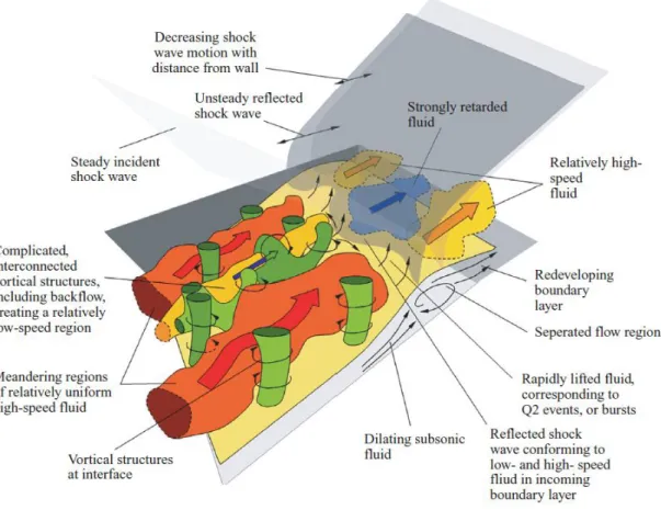
Fig. 7.1 Conceptual model of shock wave turbulent boundary layer interaction.

･････ 103

(17)

表目次

第6章

Table. 1 Comparison of parameter for each calculation

･････ 89

主要記号

aij : 行列A の要素

A : 5行5列行列

c : 音速

Cf : 局所摩擦係数 cij : 一階微分行列要素 Cp : 定圧比熱

c : 一階微分行列 dij : 二階微分行列要素 d : 二階微分行列

d1,d2,d3,d4,d5 : 特性波解析におけるベクトル要素 dc : 特性波解析におけるベクトル

D, D² : y方向（主流垂直方向），一階および二階微分演算子 dˆ3D : 固有関数

ET : 全エネルギー

f : 周波数

F : 流束ベクトル

k : 波数

k1 : 主流方向波数 k3 : スパン方向波数

Lx : x方向（主流方向）計算領域長さ Ly : y方向（主流垂直方向）計算領域長さ Lz : z方向（スパン方向）計算領域長さ L1,L2,L3,L4,L5 : 特性波振幅

M : 代表マッハ数，主流マッハ数 N : 格子点数，モード数

Nx : x方向（主流方向）格子点数

(18)

Ny : y方向（主流垂直方向）格子点数 Nz : z方向（スパン方向）格子点数

p : 圧力

pw : 壁面圧力 Pr : プラントル数

qj : 熱流束

Q : 速度勾配テンソルの第二不変量 Q : 従属変数ベクトル

Re : レイノルズ数

t : 時間

T : 温度

u ( = u1) : x方向（主流方向）速度 u_τ : 摩擦速度

U_∞ : 無限遠方における主流速度，代表主流速度 x ( = x1) : 主流方向座標

y ( = x2) : 主流垂直方向座標 z ( = x3) : スパン方向座標

v ( = u2) : y方向（主流垂直方向）速度 w ( = u3) : z方向（スパン方向）速度 α : 主流方向の波数

αC, αD : コンパクトスキームにおける係数 β : スパン方向の波数

βC, βD : コンパクトスキームにおける係数

γ : 比熱比

δ* : 排除厚さ δθ : 運動量厚さ

θ : 三次元モードと二次元モードのなす角度 λi : 特性速度

μ : 粘性係数 ν : 動粘性係数

ρ : 密度

τij : 粘性応力 ωx : 主流方向渦度 ωy : 主流垂直方向渦度 ωz : スパン方向渦度

ω : 固有値

ωi : 線形性成長率，ωの虚部 ωr : 角周波数，ωの実部

(19)

subscription / superscription

Δ・ : ・の間隔

・* : ・の無次元量

・' : ・の変動量

・_∞ : 無限遠方における・

・_rms : ・に対するR.M.S.値

・₀ : ・の流入部における値

・⁺ : 摩擦速度u_τと動粘性係数νで無次元化した・の壁スケール

・_vd : Van-Driest変換した・の値

・ : ・のアンサンブル平均値

・~

: ・のファーブル平均値

(20)

第 1 章緒言

1.1 研究背景

超音速・極超音速流れにおいて，流れの偏向に伴い衝撃波が発生する．そのため，衝撃波/境界層干渉 ( 本論文ではSWBLIと略記する ) は航空宇宙工学でよく観察される現象であり，圧縮機などの流体機械分野でも基本的課題となる．例えば，スペースプレーンに用いられるスクラム/ラムジェットエンジンや超音速機ターボジェットエンジンの空気取入口 ( インテーク ) において，

インテーク内の高速流れの中に発生する衝撃波の挙動がエンジンの性能に重大な影響を与える．

一方，SRB ( Solid Rocket Booster：固体補助ロケット) を有するロケットなどでは，打ち上げの際にSRBから生じた衝撃波がロケット本体表面に発達した境界層に入射することによって，局所的な圧力上昇や空力加熱を引き起こすことが知られている．このように，超音速や極超音速で飛行する飛翔体などでは，飛翔体表面に発達する境界層と衝撃波との干渉が起こり，局所的な加熱や境界層剥離などが生じて飛翔体の飛行特性を著しく変化させる．さらに，衝撃波の低周波数振動

( low-frequency unsteadiness ) による航空機機体の疲労損傷なども重要な問題である．

衝撃波はＥ.Mach ( 1887 ) がシャドウグラフ法によってその存在を示すまでは，想像上の概念として扱われていた．この結果の出現と産業革命における蒸気タービンなど工学的な需要とが重なり圧縮性流体力学への関心は急激に高まった．そして，Ferri ( 1940 ) が高速風洞における翼周り流れの観察からSWBLIに関する論文を初めて発表した．その後も数々の研究者によって SWBLI の研究は続けられてきたが，Ferri ( 1940 ) の研究から半世紀以上たった現在においてもSWBLIに対する空気力学的な関心は尽きることなく続いている ( Humble ( 2008 ) ) ．

SWBLI研究が始まった初期には実験により目覚ましい成果 ( 1.3.1節参照 ) が挙げられた．し

かし，近年のコンピュータ環境の急速な発展の恩恵による，Direct Numerical Simulation ( DNS ) や Large Eddy Simulation ( LES ) さらにはLESとReynolds-Averaged Navier-Stokes ( LES-RANS ) のハイブリットといった高精度を有した数値計算 ( 1.3.2節参照 ) の発展やPIVなどの実験計測法の新たな開発により，更なる発展を遂げようとしている．

1.2，1.3節述べるようにSWBLI研究の中で膨大な成果が積み上げられてきたが，衝撃波の低周

波数振動や衝撃波と干渉する層流境界層の遷移など依然として未解明の現象も多く残されている．

衝撃波の低周波数振動に関する研究に比べ，超音速境界層の遷移形態に関する研究は尐なく，中でも衝撃波と干渉する層流境界層の乱流遷移に関する研究は非常に尐ない．衝撃波と干渉する層流境界層の乱流遷移構造に着目しているところが本研究における一つの特徴である．

本研究では高精度シミュレーションをSWBLIの調査に用いる．このSWBLIに関する高精度シミュレーションによる研究は，流れの理解を深め，正確なデータベースを提供することにより次世代航空宇宙輸送機設計の改良や乱流モデルの開発に対し重要な役割を担っている．一方，SWBLI のような衝撃波を伴うような流れについては，現代の流体力学計算技術では非常に多くの格子点を要し，膨大な計算時間を要する．そのため，ロバストであり高精度なシミュレーションスキームについては，現在でも盛んに研究が進められている．しかし，本研究では衝撃波を伴うような流れについては現時点での先端的スキームを使い，衝撃波を伴う境界層の乱流遷移構造について

(21)

解析することを第一の目的としている．そのため，SWBLIに対するスキームの比較や評価については議論の対象とはしない．

1.2 SWBLI の分類

衝撃波を伴う境界層は大きく分けると次のような二つに分類される．( Délery & Dussauge ( 2009 ) )

二次元干渉：境界層とそれに従う衝撃波構造が基本的に二次元的に構成されるもの．

圧縮ランプによって形成される衝撃波

入射衝撃波発生機器 ( 二次元corner/fin等 ) によって形成される斜め衝撃波遷音速流れでみられる垂直衝撃波

バックステップおよびフォーワードステップ流における剥離に伴う衝撃波圧力ジャンプによる圧縮性不連続

三次元的干渉：障害物によって形成される衝撃波

Swept wedge/corner/step Blunt/Sharp fin

研究背景でも述べたように，本研究では衝撃波を伴う超音速乱流遷移境界層の流れの特徴を調査することを目的としている．加えて，物理的な現象に類似点が多いため圧縮ランプによる干渉についても衝撃波/乱流境界層干渉に関する主要な現象に限って触れる．これらの二つの形式による衝撃波の研究はこれまでにも数多く行われており．以下にこれまでに明らかとなっているこれら二つの流れの特徴について概説する．

1.2.1 圧縮ランプによって形成される衝撃波

圧縮ランプ上にできる境界層の問題は，衝撃波を伴う境界層の問題の中で実験が容易に行えるという利点もあって，半世紀以上前から盛んに研究が行われてきた分野である． ( Ardonceau ( 1984 ), Smits & Muck ( 1987 ), Andreopoulos & Muck ( 1987 ), Selig et al. ( 1989 ), Erengil & Dolling ( 1991 ), Adams ( 2000 ), Beresh et al. ( 2002 ) , Ganapathisubramani et al. ( 2007 ) , Bookey et al.

( 2005 ) ,Wu & Martin ( 2007, 2008 ) ) .

これらの流体力学的な問題は，機体の幾何学形状やフラップによる流れの偏向などの流れの不連続性に起因した工学上よく起きる問題である．衝撃波は壁面の傾斜による流体の圧縮変動が原因として生じるため，圧縮ランプの傾斜角が重要なパラメータとなる．

(22)

Fig. 1.2.1 The structure of a ramp flow without boundary layer separation. Adapted from Arnal & Délery ( 2004 )

ランプの傾斜角β が小さい時には，流れ場全体としての構造はランプの足元で起こる干渉の影響はあまり受けない．大きく影響を受けるのは，壁面圧力分布でありランプ上流の圧力p0に対しその下流の圧力p1は急激に増加することが非粘性の斜め衝撃波方程式から導ける．このとき壁面圧力分布は，" upstream influence " メカニズムを表す．" upstream influence " とは衝撃波の影響をコーナーの先端よりどの程度上流で感知するかということで，図1.2.1で流線が偏向し始める点を指す．このことは，図1.2.1に示すように亜音速領域が境界層内に存在することを示しており，この亜音速領域が存在することにより上流，下流のどちらにも撹乱が伝播する．この亜音速領域の厚さや衝撃波 ( 圧力波 ) の発生位置はランプ上流の流れの状態に大きく依存しており，レイノルズ数またはマッハ数が十分に高ければ，ほとんどの領域が非粘性領域となり亜音速領域は境界層内の非常に薄い領域のみに存在することになる．このようなケースでは，壁面に非常に近いところで衝撃波が発生することになり，圧力や慣性力に対して粘性力が無視できないような急速な干渉が起こるという特徴を有している．これらの干渉は " Triple-deck theory " としてまとめられている ( Lighthill ( 1953 ) )．一方，ランプ傾斜角βが大きくなると，upstream influenceを受ける領域が大きくなり，剥離を引き起こすのに十分な圧力上昇が発生する ( 図 1.2.2 参照 )．この剥離が起こると再付着の ( すなわち，流れがランプの傾斜と平行に流れるようになる ) 際に第二の衝撃波 ( 再付着衝撃波 ) が発生する．再付着衝撃波と剥離衝撃波は壁面から離れた非粘性領域の点④ おいて収束し，この点④より下流に二つの反射衝撃波を形成し，その間に滑り面を形成する．この面の上下面において物理量は一致せず上流と同様の関係を保ったまま下流へと流れる．

(23)

Fig. 1.2.2 The structure of a ramp flow with boundary layer separation. Adapted from Arnal & Délery ( 2004 )

1.2.2 入射衝撃波発生機器によって形成される斜め衝撃波

このタイプの衝撃波は，入射衝撃波発生機器によって形成される平面的な斜め衝撃波が境界層と干渉し，そして，入射衝撃波の角度に合った反射衝撃波を形成する．工学的には，スペースプレーンに用いられるスクラム/ラムジェットエンジンや超音速機ターボジェットエンジンの空気取入口 ( インテーク ) において，インテーク内の高速流れの中に発生する衝撃波の挙動がエンジンの性能に重大な影響を与える．入射衝撃波発生機器による衝撃波は，圧縮性ランプとは違い，

ランプによる流線の曲率を考える必要がないため，近年，工学的にも学術的にも注目されている分野である．初期の研究は，Green ( 1970 ) によって詳述されている．一方，近年のこの分野における新たな発展や知見についてはDélery & Marvin ( 1986 )，Smits & Dussauge ( 2006 )，Dussauge et

al. ( 2005, 2009 ) が詳細なレビューをしている．近年行われた実験，数値計算にはBack & Cuffel

( 1976 )，Deleuze ( 1995 )，Garnier et al. ( 2002 )， Bookey et al. ( 2005 )， Priebe et al. ( 2009 )，Piponniau et al. ( 2009 )，Touber & Sandham ( 2009 ) などが挙げられる．

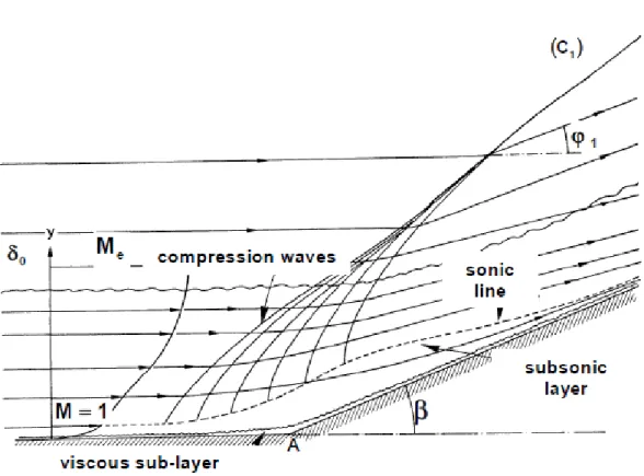
入射衝撃波による圧力勾配の大きさが十分でないときには，境界層剥離は生じない．剥離を伴わないケースの概念図を図1.2.3に示す．入射衝撃波 ( C₁ ) が境界層に侵入していることが確認できる．ここでは，局所マッハ数が下がり，境界層が急激に曲げられる．このとき入射衝撃波の強度が比較的弱ければ，衝撃波は音速ラインに達すること無く消滅してしまう．同時に，入射衝撃

(24)

Fig. 1.2.3 The structure of impinging-reflecting shock without boundary layer separation. Adapted from Arnal & Délery ( 2004 )

Fig. 1.2.4 Mean wall-pressure distribution for a SWBLI, demonstrating the influence of shock upstream of its inviscid origin. Adapted from Délery & Dussauge ( 2009 )

(25)

Fig. 1.2.5 The structure of impinging-reflecting shock with boundary layer separation. Adapted from Arnal & Délery ( 2004 )

波の影響は境界層の曲げられた領域に生じる亜音速領域を通じて上流へと伝わり圧力の上昇を引き起こす．図1.2.4に示すように，壁面圧力分布は非粘性解よりも上流から上昇をはじめ，そして，

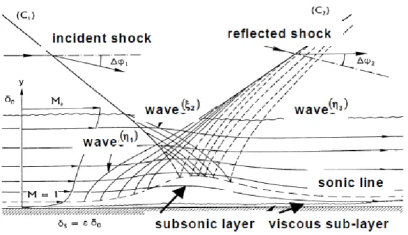
より下流において非粘性解と同様の圧力まで上昇する．このケースでは，非粘性解と粘性解に大きな差異は見られない．このように粘性の影響をあまり受けないような干渉の振る舞いをするとき，それを弱い干渉と呼ぶ．境界層内の亜音速領域の膨張は超音速領域に影響を与え，圧縮ランプと同様，圧縮波 ( η1 ) を発生し，その後再付着領域から発生した圧縮波 ( η3 ) と交差し反射衝撃波 ( C₂ ) を形成する．境界層内にどの程度の亜音速領域が形成され，upstream influenceをどの程度受けるかについては，入射衝撃波の強さだけではなく，上流の流れの状態にも強く依存する．

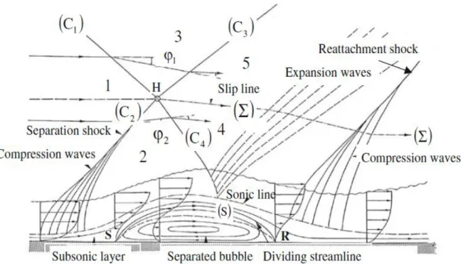
一方，入射衝撃波の強度を強くしていくと圧縮ランプのケースと同様，境界層剥離を生じるようになる．剥離を伴うケースの概念図を図1.2.5 に示す．図 1.2.5 には剥離点 S 後方に分離流線

( S ) を形成し，再循環している剥離泡が形成される．剥離泡による流線 ( S ) は剥離点 S に始ま

り，再付着点 R で終了する．剥離点 S 後方に現れる剥離せん断層における強い混合作用により，

高速領域から剥離領域へとエネルギーの流れが生じる．結果として，再付着に伴う減速が起こるまで，分離流線 ( S ) の流速 U_Dは増速し続ける．入射衝撃波は剥離した粘性流にまで浸入する．

ここでは，圧力上昇が一定となっているためにexpansion fan が発生する．このexpansion fanの発生により流れの偏向が起こり急速に再付着領域へと流れが進み，再付着点 R において流れは再付着する．上述の圧縮ランプのケースにおける過程と同様に剥離領域の外部では，圧力波が形成されており壁から離れた領域において収束し，反射衝撃波を形成する．

(26)

Fig. 1.2.6 Wall pressure distribution, in shock separated flow Adapted from Délery & Dussauge ( 2009 )

図1.2.6に示すように，壁面圧力分布は最初に剥離に伴う急激な上昇をした後，剥離領域においては一定な値をしばらく取り，再付着領域に向けて再び急激な圧力上昇をする．このケースは非粘性解と比べて著しく差異のあるケースであり，強い粘性－非粘性干渉と呼ばれる．この意味は，

流れの解析において粘性の効果を十分に考慮しなければならず，粘性効果は非粘性解を尐し調整する程度ではなく，このケースでは解の形成に中心的な役割を果たすということである．

1.3 SWBLIのこれまでの研究

このセクションではこれまでの研究において解明されてきた SWBLI のキーポイントについて簡単に概観する．境界層と衝撃波の干渉により流れ場も乱流特性も大きく影響を受ける．そのため，この複雑な現象を解明するためにこれまでに多くの実験，数値計算による研究がおこなわれてきた．これまでに発表された論文は多種多様である．よって，全てを網羅することはできないが，衝撃波の干渉を伴う境界層の流れのダイナミクスにおいて，現在重要とされているものを取り上げる．

(27)

Fig. 1.3.1 Wall-pressure distribution for laminar separation for various model configurations and Reynolds number at M = 2.3. Adapted from Chapman et al. ( 1957 )

1.3.1 実験によるSWBLI研究

壁面摩擦係数と壁面圧力分布を調べることは，干渉領域を知る上で非常に重要である．そのため，早くからこの分野では研究の対象となってきた．Chapman et al. ( 1957 ) は層流から乱流まで非常に多くの実験を通して，圧力と干渉領域の大きさに対する適切なスケーリングを発見し，そこから " free-interaction " と呼ばれる概念を考案した．このスケーリングはマッハ数と上流境界層の物理量から導かれるものであり，圧縮ランプやフォーワードステップにおいて様々なレイノルズ数に対し成り立つことを示している ( 図1.3.1 ) ．一方，Shang et al. ( 1976 ) は，圧縮ランプと入射衝撃波発生機器によって形成される衝撃波による干渉を比較し，圧縮ランプの傾斜角が入射衝撃波発生機器による入射角の2倍程度であるとき壁面圧力分布がよく一致することを確認した．しかし，Smits & Dussauge ( 1996 ) によるとこれらが成り立つのは，上流の流れ場が定常な層流状態のときだけであり，非定常な時にはこの判断基準には合致しないことを指摘している．

Settles et al. ( 1979 ) は，傾斜角をもった圧縮ランプを用いてこの非定常性に着目した研究を行

った．ここでは，壁面ストリークパターン ( 図1.3.2 ) の干渉領域における様子を観察することにより，流れの三次元性について言及した．さらに，再付着領域における流れの平均場にも着目し，

回復領域が干渉点に対しどの程度下流まで続くかについて言及した．

壁面圧力変動の解析により衝撃波の壁近傍での挙動 ( 図1.3.3 ) の詳細を報告したのがDolling

et al. ( 1983, 1985 ) である．衝撃波は平均位置の近傍において低周波数，高強度の圧力変動を有す

ることを確認した．また，衝撃波の振動の挙動は衝撃波の強度に依存していることも明らかにした．

(28)

Fig. 1.3.2 Surface streak patterns for compression corner flows at Mach 2.9. Adapted from Settles et al.

( 1979 )

Smits & Muck ( 1987 ) は主流方向質量流束と重みづけレイノルズ応力を精巧な実験を行うこと

により初めて示した．干渉に伴い壁面から遠方までの広範囲に及ぶ大規模で非等方的な撹乱の成長が生じていることを示し，それらの最大値は圧力の上昇に比例していることも確認した ( 図

1.3.4 ) ．Kuntz et al. ( 1987 ) は，壁面垂直方向の計測に成功し，剥離領域と再付着領域の平均分布

についてより詳細な結果を報告した．

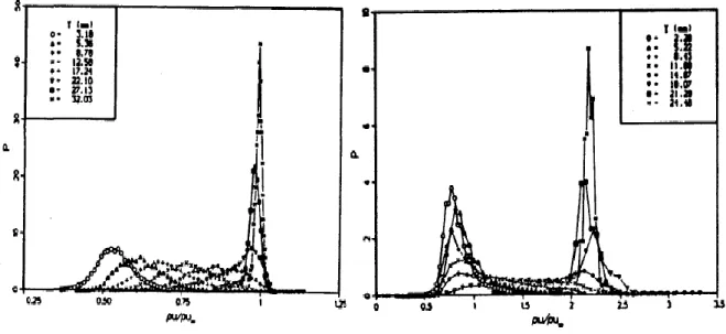
Selig et al. ( 1989 ) は干渉領域における質量流束の確率密度を報告した ( 図1.3.5 )．この研究で

は干渉点上流では，ほぼガウシアン分布をしており乱流境界層分布と変わらないが，干渉点下流では二つのピークをもつ分布となることを示した．この分布は干渉点下流の変曲点をもつ速度分布の不安定性を表している．一方，この研究では，衝撃波の非定常性による剥離領域についての影響はなかったと報告している．

Beresh et al. ( 2002 ) は上流の境界層の条件に対する干渉領域における衝撃波の非定常性につい

て調査を行った．この調査では上流の境界層内部の主流速度変動が正の値を示す時，衝撃波の位置は下流側にずれ，逆に負の値を示す時は上流側にずれるといった強い相関関係があることが確認された．その特性周波数は，上流の乱流境界層 ( 40KHz ) に対して一桁程度低い周波数である

4 ~ 10 KHz程度であることが発見された．この論文では，上述のメカニズムを簡単なモデルを用

いて説明している ( 図1.3.6 )．このモデルによると乱流境界層において正の変動を示す時，速度分布は，壁面近傍まで満たされた状態となりその結果として，衝撃波は下流方向へ押しこまれる状態となる．逆に負の変動を取るときにはこの逆のメカニズムが働くと説明した．さらに，この

(29)

Fig. 1.3.3 Wall pressure time-histories. Adapted from Dolling& Or ( 1985 )

Fig. 1.3.4 ( a ) to ( c ) demonstrate the longitudinal Reynolds stress evolution along interaction region for 8°, 16°and 20°compression corner angles. Adapted from Smits & Muck ( 1987 )

(30)

( a ) upstream of the interaction point ( b ) downstream of the interaction point

Fig. 1.3.5 Probability density function of the muss-flux profile. Adapted from Selig et al. ( 1989 )

Fig. 1.3.6 Relationship between incoming boundary layer and separation shock foot unsteadiness. Adapted from Beresh et al. ( 2002 )

(31)

Fig. 1.3.7 Power spectral densities around the reflected shock with varying incident shock strength.

Adapted from Dupont et al. ( 2006 )

モデルについてはGanapathisubramani et al. ( 2007 ) がPIVを用いて調査し，乱流境界層において発見されている超大規模構造の概念 ( Adrian ( 2007 ) ) と関連させ，より詳細な議論をしている．

Dupont et al. ( 2006 ) は衝撃波の強さを変えながら斜め衝撃波の組織構造についての調査を発表

した．干渉領域における時間的，空間的スケール ( 反射衝撃波の周波数，干渉領域の距離，衝撃波の可動域の距離 ) をいくつかの偏向角のケースについて解析し，その結果を示した．反射衝撃波の周波数は，偏向角に多尐依存するが上流乱流境界層の周波数に対しストローハル数で一桁程度低い周波数 ( St = 0.025 ~ 0.04, 図1.3.7 ) であり，境界層厚さからその2倍程度の距離を主流方向に動くことが可能であることを示した．衝撃波と干渉領域の関係についても言及し，反射衝撃波の周波数と同程度の周波数で運動する，スパン方向において互いに反対方向に回転する一組の渦構造を発見した．これらの内容は，Dussauge & Dupont ( 2005 ) においても詳しくレビューされている．

Humble et al. ( 2009a, 2009b ) はトモグラフィー PIVと熱線流速計を用い斜め衝撃波と超音速乱

流境界層の干渉について調査した．上述した衝撃波と高速領域および低速領域との干渉について三次元的に解析し，反射衝撃波面が主流方向には並進しスパン方向にさざ波構造を形成していることを明らかにした ( 図 1.3.8 ) ．また，POD ( Proper Orthogonal Decomposition ) による解析では，

上流の境界層の状態と剥離泡，反射衝撃波の位置に対する弱い相関関係を見つけ，上流の低速領域に存在するヘアピンパケット構造との関係にも言及した．

Piponniau et al. ( 2009 ) はPIVを用いて反射衝撃波の低周波数変動の調査を行い，反射衝撃波の

低周波数変動を再付着領域付近に現れる混合層と剥離泡の伸縮について関連付け，これらをモデル化し，これがPIVによる観測結果とよく一致することを確認した．

(32)

Fig. 1.3.8Schematic representation of the three-dimensional physical model. Adapted from Humble et al.

( 2009a )

1.3.2 数値計算によるSWBLI研究

これまでに見てきた数多くの実験による研究とともに，コンピュータ環境の急速な発展により数値計算もSWBLI のような問題解明に当たり重要なツールのひとつとなった．SWBLI は Direct Numerical Simulation ( DNS ) や Large Eddy Simulation ( LES ) さらにはLESとReynolds-Averaged

Navier-Stokes ( LES-RANS ) のハイブリット法などの一定以上の精度を有した数値計算により正

確な流れ場を再現できるようになった．それだけではなく，干渉領域のような非定常場の流れの三次元的な詳細を理解するためにも重要なツールとなっている．しかしながら，乱流を計算するのに有効な精度を有するためには，現在のところ直接計算では，低から中程度のレイノルズ数の範囲に限られている．Knight & Degrez ( 1998 ) は衝撃波/乱流境界層の予測に対して RANS はどの程度合致しているのかについて調査し，壁面圧力と熱伝導についてはよく一致していることを確認した．近年の Edwards ( 2008 ) によるレビューでは DNS，LES，LES-RANS による SWBLI 予測に対して可能な点と限界について議論がなされており，SWBLI の重要な特性を明らかにする潜在的な能力を直接計算は秘めているという結論を発表している．

Adams ( 2000 ) は傾斜角 18°，Mach 3 の圧縮ランプについての DNS を行った．ここでは予備

の乱流境界層計算を行い，流入条件として用いた．210δ0 / U_∞ という長さの時間平均を取り，後流のような速度分布と衝撃波により増幅されたレイノルズ応力を示した．さらに深い議論により

(33)

圧縮性の影響は無視できなくなり Strong Reynolds Analogy ( SRA ) は成り立たないことを示した．

また，衝撃波の振動周波数は流入する乱流境界層のバースティング周期と同程度であるという結果も示した．

Garnier ( 2002 ) はフィルターを利用した数値計算を行った．壁乱流によく一致する " mixed grid

subscale model " を用い，さらに，流入条件には " recycling-rescaling " 法を圧縮性に対応するように改良し，利用した．Deleuze ( 2003 ) による実験を模擬し入射角 8°，Mach 2.3 という条件で計算を行い，実験と干渉流域前後における温度や流速等の平均量，二乗平均平方根がよく合うことを示した．また，壁面摩擦係数，排除厚さ，境界層厚さについてもよく一致する結果を示した．

しかしながら，平均時間の制限から衝撃波の振動周波数を確認することはできなかった．

Bookey et al. ( 2005b ) は圧縮ランプ ( 傾斜角24° ) と入射衝撃波発生機器によって形成される

斜め衝撃波 ( 入射角12° ) についてMach 2.9 に対してのDNSを行い，Bookey et al. ( 2005a ) が計算と同程度のレイノルズ数で行った実験結果との比較を発表した．二次元の平均密度場を基に実験とよく一致する衝撃波構造を計算から導けていることを確認し，よりレイノルズ数の高い

Selig et al. ( 1989 ) による実験と比較し，結果が類似していることを確認した．質量流束の乱流強

度は，実験による誤差を考慮すると非常によく一致しており，また，壁面摩擦係数の値の大きさについてはレイノルズ数が異なるため，差異がみられたがその剥離領域の大きさについてはよく一致していた．すなわち，剥離領域の大きさはレイノルズ数に対し独立であると結論付けた．圧縮ランプについては，壁面の曲率効果による三次元構造を観測したが，一方，入射衝撃波のケースでは三次元構造を観測できなかった．

Pirozzoli et al. ( 2005 ) は，Deleuze ( 2003 ) による実験を模擬し入射角 8°，Mach 2.25 という条件で空間発展型DNSを行った．ここでは，recycling-rescaling 法といった特別な流入条件は使われておらず，遷移と境界層発達を完全に加味した計算となっている．まずこの論文では，干渉領域の理解を深めるため平均場，乱流場についての非常に豊富なデータが示されている．干渉領域から十分離れた上流，下流の点では，乱流統計量が密度の重みを付けることで非圧縮性乱流境界層の結果とよく一致することを示し，完全な乱流境界層へと回復するためには境界層厚さの10倍のオーダーの距離が必要だと主張している．剥離領域における渦構造について詳しく報告し，さらに，これらの構造によって衝撃波の足元が下流へと押し流されていることを示した．これらの観測から，音響共鳴を仮定し，衝撃波と渦構造の干渉によって発生した音波が上流へと伝わり，剥離泡を振動させ，その結果，反射衝撃波を振動させるという一連の過程を提案した．

Loginov ( 2006 ) はApproximate Deconvolution Model ( ADM ) ( Stolz et al. ( 2001 ) ) を用いた非常に高解像度なLESによる圧縮ランプ ( 傾斜角25°，Mach 2.95 ) の計算を行い，瞬間場，平均場に

ついてZheltovodov et al. ( 1990 ) との比較を示した．壁面摩擦係数，壁面圧力の分布はよく一致し

ており，さらに，質量流束，密度，流速変動，壁面圧力変動についてもよく一致することを示した．圧力変動の確率密度関数を用いた解析では，Dolling & Murphy ( 1983 ) により観測された，衝撃波の高い間欠率のために起こる干渉領域での確率密度のダブルピークについてもよく再現できることを示した．衝撃波による乱流強度の増加についての議論をし，その原因を干渉領域におけるゲルトラータイプの渦であると結論付けた．

さらに，圧縮ランプ ( 傾斜角 24°，Mach 2.9 ) において広範囲な結果を示し Bookey et al.

( 2005 ) による実験結果との比較を議論したのがWu & Martin ( 2007, 2008 ) である．上流境界層