自然現象の写実的表現モデルの研究

東京電機大学

博 士 論 文

自然現象の写実的表現モデルの研究

Visual Simulation Models for Natural Phenomena

2018

年

3

月

第 5 章 結論 69 5.1 本研究のまとめ . . . 69 5.2 今後の展開 . . . 70 5.2.1 大気光学現象の再現手法 . . . 70 5.2.2 ウェザリング現象の再現手法 . . . 71 謝辞 72 参考文献 73 付 録 A 四角い太陽蜃気楼 (拡大画像) 78 付 録 B さまざまなジオメトリでの錆の成長過程 (拡大画像) 84 付 録 C 人間の知覚特性の考慮に関する検討 100 C.1 Introduction . . . 100 C.2 Related Works . . . 101

C.2.1 Optical System Approach . . . 101

C.2.2 Neural System Approach . . . 102

C.3 Visual Simulation Method . . . 102

C.3.1 Optical Simulation Step . . . 103

C.3.2 Neural Simulation Step . . . 107

C.4 Experimental Results . . . 111

C.4.1 Snellen Chart . . . 111

C.4.2 Hermann Grid Illusion . . . 113

C.4.3 Direction Boards . . . 113

C.5 Concluding Remarks . . . 114

付 録 D 研究業績一覧 118 D.1 査読付き論文 ( Journal Papers ) . . . 118

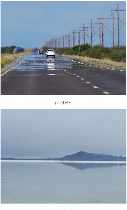
(a) 逃げ水

(b) 浮島現象

(a) ファータモルガナ

(b) 四角い太陽

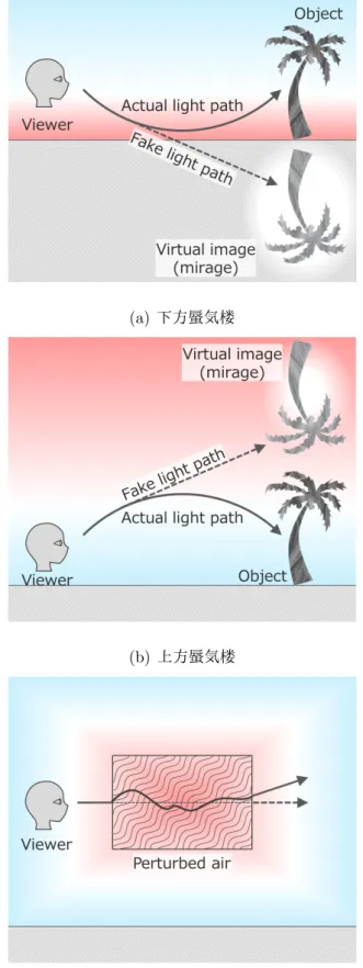
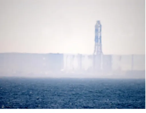
(a) 下方蜃気楼

(b) 上方蜃気楼

(c) 大気の摂動

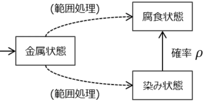
この方法に従うと，摂動のためのシステム行列 TP は以下のように表現される． T_PE =    e ψϵ 0t ₁    (3.10) ここで e は 4× 4 の単位行列，0 は 4 次元の列ゼロベクトル，ψϵは 3.4.2 項で議論し たノイズレイベクトルである.

3.5

結果

3.5.1

実験環境

(a)

(b)

(a)

(b)

(a)|⃗d| = 0.0

(b) |⃗d| = 0.5

(c) |⃗d| = 1.0

(a) |⃗d| = 0.0

(b) |⃗d| = 0.5

(c) |⃗d| = 1.0

表 4.3: 実験環境

図 4.8: 生成された腐食過程 (形状: 平面)

図 4.9: 生成された腐食過程 (形状: 半円柱)

(a) 実際の写真

参考文献

[1] M. Berger, T. Trout, and N. Levit. Ray tracing mirages. Computer Graphics

and Applications, IEEE, 10(3):36–41, May 1990.

[2] F.K. Musgrave and M. Berger. A note on ray tracing mirages (comments and author’s reply). Computer Graphics and Applications, IEEE, 10(6):10–12, November 1990.

[3] Eduard Gr¨oller. Nonlinear ray tracing: Visualizing strange worlds. The Visual

Computer, 11:263–274, 1995.

[4] Jos Stam, Eric Languenou, and Projet Syntim. Ray tracing in non-constant media. In Eurographics Workshop on Rendering, pages 225–234, 1996.

[5] F.J. Seron, D. Gutierrez, G. Gutierrez, and E. Cerezo. Visualizing sunsets through inhomogeneous atmospheres. In Computer Graphics International, pages 349–356, June 2004.

[6] Y. Zhao, Y. Han, Z. Fan, F. Qiu, Y.-C. Kuo, A.E. Kaufman, and K. Mueller. Visual simulation of heat shimmering and mirage. Visualization and Computer

Graphics, IEEE, 13(1):179–189, January 2007.

[7] Ken Perlin. An image synthesizer. SIGGRAPH Comput. Graph., 19(3):287– 296, July 1985.

[8] Greg Turk. Generating textures on arbitrary surfaces using reaction-diffusion.

[9] Julie Dorsey, Hans Køhling Pedersen, and Pat Hanrahan. Flow and changes in appearance. In Proceedings of the 23rd Annual Conference on Computer

Graphics and Interactive Techniques, SIGGRAPH ’96, pages 411–420, New

York, NY, USA, 1996. ACM.

[10] Yanyun Chen, Lin Xia, Tien-Tsin Wong, Xin Tong, Hujun Bao, Baining Guo, and Heung-Yeung Shum. Visual simulation of weathering by γ-ton tracing. In

ACM SIGGRAPH 2005 Papers, SIGGRAPH ’05, pages 1127–1133, New York,

NY, USA, 2005. ACM.

[11] Henrik Wann Jensen. Global illumination using photon maps. In Proceedings of

the Eurographics Workshop on Rendering Techniques ’96, pages 21–30, London,

UK, UK, 1996. Springer-Verlag.

[12] Julie Dorsey and Pat Hanrahan. Modeling and rendering of metallic patinas. In Proceedings of the 23rd Annual Conference on Computer Graphics and

In-teractive Techniques, SIGGRAPH ’96, pages 387–396, New York, NY, USA,

1996. ACM.

[13] Stephane Merillou, Jean-Michel Dischler, and Djamchid Ghazanfarpour. Cor-rosion: Simulating and rendering. In Proceedings of the Graphics Interface 2001

Conference, pages 167–174, June 2001.

[14] Tomokazu Ishikawa, Kousaku Kamata, Yuriko Takeshima, and Masanori Kaki-moto. Rusting and corroding simulation taking into account chemical reaction processes. In ACM SIGGRAPH 2016 Posters, SIGGRAPH ’16, pages 65:1– 65:1, New York, NY, USA, 2016. ACM.

Vi-sion Graphics and Image Processing, ICVGIP ’14, pages 38:1–38:8, New York,

NY, USA, 2014. ACM.

[16] St´ephane Gobron and Norishige Chiba. Crack pattern simulation based on 3d surface cellular automaton. In Proceedings of the International Conference on

Computer Graphics, CGI ’00, pages 153–, Washington, DC, USA, 2000. IEEE

Computer Society.

[17] Tien-Tsin Wong, Wai-Yin Ng, and Pheng-Ann Heng. A geometry dependent texture generation framework for simulating surface imperfections. In

Pro-ceedings of the Eurographics Workshop on Rendering Techniques ’97, pages

139–150, London, UK, UK, 1997. Springer-Verlag.

[18] Murray Eden. A two-dimensional growth process. In Proceedings of the Fourth

Berkeley Symposium on Mathematical Statistics and Probability, Volume 4:

Contributions to Biology and Problems of Medicine, pages 223–239, Berkeley,

Calif., 1961. University of California Press.

[19] E. Somfai, L. M. Sander, and R. C. Ball. Scaling and crossovers in diffusion limited aggregation. Phys. Rev. Lett., 83:5523–5526, Dec 1999.

[20] A. Taleb, A. Chauss, M. Dymitrowska, J. Stafiej, and J. P. Badiali. Simulations of corrosion and passivation phenomena: diffusion feedback on the corrosion rate. The Journal of Physical Chemistry B, 108(3):952–958, 2004.

[21] Haitao Wang and En-Hou Han. Cellular automata modeling on corrosion of metal with line defects. International Journal of Electrochemical Science, 10(1):815–822, January 2015.

[22] Turner Whitted. An improved illumination model for shaded display.

[23] Mikio Shinya, T. Takahashi, and Seiichiro Naito. Principles and applications of pencil tracing. SIGGRAPH Comput. Graph., 21(4):45–54, August 1987. [24] Ryoma Tanabe, Tomoaki Moriya, and Tokiichiro Takahashi. A generation

method of rust aging texture considering rust spreading. In Proceedings of

2015 Joint Conferenct of IWAIT and IFMIA, 2015.

[25] Herbert H Uhlig and R Winston Revie. Corrosion and Corrosion Control, 3rd

edition. Wiley Interscience, 1989.

[26] Johnson. N.L. Systems of frequency curves generated by methods of translation.

Biometrika, 36(1/2):149–176, January 1949.

[27] S. Mostafawy, O. Kermani, and H. Lubatschowski. Virtual eye: retinal image visualization of the human eye. IEEE Computer Graphics and Applications, 17(1):8–12, Jan 1997.

[28] M. Yoshida, H. Kaneko, and K. Onuma. The simulation eyesight using psf analyzer. In Meeting abstract of 13th annual meeting Japanese Academy of

Optometry and Ophthalmic Science, 2009.

[29] Brian A. Barsky. Vision-realistic rendering: Simulation of the scanned foveal image from wavefront data of human subjects. Applied Perception in Graphics

and Visualization, 2004.

[30] Kunihiko Fukushima. A feature extractor for curvilinear patterns: a design suggested by the mammalian visual system. Kybernetik, 7(4):153–160, Sep

1970.

[31] James A. Ferwerda, Sumanta N. Pattanaik, Peter Shirley, and Donald P. Green-berg. A model of visual adaptation for realistic image synthesis. In Proceedings

of the 23rd Annual Conference on Computer Graphics and Interactive

[32] Y. Kobayashi and T. Kato. A high fidelity contrast improving model based on human vision mechanisms. In Proceedings IEEE International Conference on

Multimedia Computing and Systems, volume 2, pages 578–584 vol.2, Jul 1999.

[33] De Monasterio F. M. and P. Gouras. Functional properties of ganglion cells of the rhesus monkey retina. The Journal of Physiology, 251(1):167–195, Sep 1975.

[34] Ophthalmic optics – visual acuity testing – standard optotype and its presen-tation. Standard, International Organization for Standardization, Jul 2009. [35] Optics and optical instruments – visual acuity testing – method of correlating

optotypes. Standard, International Organization for Standardization, Sep 1994. [36] Visual acuity testing equipment. Standard, Japanese Industrial Standards

付 録

_A

四角い太陽蜃気楼

₍

拡大画像

₎

本章では表 A.1 の結果画像の拡大版を掲載する．それぞれの対応は表 A.1 の通り である．

付 録

_C

人間の知覚特性の考慮に関す

る検討

本章では，本論文で提示したようなビジュアルイメージを人間の視覚特性を考慮 して提示する手法について詳述する．

C.1

Introduction

This is because the designer’s viewpoint and visual angle to the computer monitor are different from viewer’s viewpoints and visual angle to the exhibited ob-ject. Since the distance between the designer and the computer monitors is very close, the designer do not notice this problem on visual appearance. On the other, the distance between the viewer and huge exhibited objects is very far. Therefore, the viewer cannot read very small characters because their viewpoints are far from the objects. If the viewers’ eyesight is weak, this problem becomes serious. Unfor-tunately, there are few design tools to simulate visual appearance considering both viewers’ viewpoint and eyesight.

to generate perceptual images. This approach can simulate various effects such as visual adaptation and eyesight caused by physiological structure of human eye.

In this paper, we propose a visual appearance simulation method of exhibited ob-jects based on image filtering approach by combining conventional two approaches. Our method can simulate visual appearance of various exhibited objects which is viewed by the viewers with arbitrary eyesight from arbitrary distant places.

C.2

Related Works

There have been proposed many methods for visual appearance simulation. These visual simulation methods are classified into two approaches: optical system approach and neural system approach.

C.2.1

Optical System Approach

In optical system, a ray from an object reaches to retina through pupil, lens and vitreous humour with complicated reflections and refractions, and finally images are formed on the retina.

There have been several simulation studies based on anatomic properties of eye. Mostafawy[27] et al proposed a method to simulate retinal image for corneal surgery. They simulated retinal image by using ray tracing technique. Their method requires various simulation parameters measured by the wavefront analyzer. Yoshida et al[28] developed a Point Spread Function (PSF) analyzer to simulate a retinal image according to optical properties of viewers’ eye. Barsky[29] proposed a similar method to generate 3D CG images.

the specific viewer based on the measured optical properties.

These conventional methods are very complicated and long-scale to simulate eye-sight, however, a simple but general method is required. Moreover, we should con-sider neural system after retinal images are simulated.

C.2.2

Neural System Approach

Neural system approach simulates visual appearance based on neural structures of human visual system. Light fallen on retina is converted to physiological stimuli, and they are propagated to brains. Stimuli fired in a retina is aggregated, enhanced and reduced through intermediate neurons. We perceive these stimuli as an image. There have been several studies based on neural system. Lateral inhibition is a phenomena caused by neural system, which neighboring neuron inhibit their reac-tion. Fukushima[30] proposed a neural network model which consisted of six-layered I/O system. Each layer behaves like a convolution filter, however, and the entire model is able to detect line segments. Ferwerda et al[31] proposed a method based on physiological studies for generating realistic images. Their methods can simulate effects such as visual adaptation and eyesight caused by physiological structure of human eye. Kobayashi and Kato[32] proposed mathematical model for simulating lateral inhibition, and applied it to natural image enhancement.

These neural system approaches are mainly intended to simulate perceptual im-ages of eyesight, but they do not consider optical system, i.e., viewers’ eyesight and visual angles.

C.3

Visual Simulation Method

we create a slide on a computer display monitor, we often zoom a figure in the slide to edit and draw its details more precisely. Such a figure is hard to read, especially, for weak eyesight viewers. We should consider visual apparent sizes of exhibited objects and viewers’ eyesight. In addition, we have to consider perceptual effects of human neural system. One of the most important properties is lateral inhibition. The lateral inhibition is a phenomena caused by the neural system. We perceive enhanced contrast of images caused by this phenomena.

We propose a visual simulation method considering both optical and neural sys-tems of human visual system. Our method consists of two steps. Each step is corresponding to one of the two systems respectively. We simulate these systems by using two convolution filters: Gaussian filter and DOG filter. These filters are applied sequentially to an input image to generate a resultant simulation image.

C.3.1

Optical Simulation Step

First step is optical simulation step, corresponds to optical system of human visual system. This step consists of two processes. First process is visual angle adjustment which fits the size of an input image to the apparent size from the viewer. Second process is an optical defocus simulation that generates blurred image. The blurred image is aimed to simulate poor eyesight. We use Gaussian smoothing filter to simulate optical blur. Parameters of Gaussian filter are measured.

Visual Angle Adjustment

図 C.1: Simulation Parameters

WR=

DRPTWI

DTPR

(C.1) Here, WI is the size of input image in pixels, DR and DT are the distance

from the viewer to real screen where simulated images are displayed and target screen(exhibited object), respectively as illustrated in Fig.C.1. PRand PT are width

and height of one pixel on the real and target screens, respectively.

Defocus Simulation

表 C.1: Experiment Environment Illuminance 610 lx

Real screen 19 inch LCD

Resolution: 1280x1024 pixels Luminace: 6.8-145.5 cd/m2

Viewer’s eyesight Over 20/20 vision Viewer’s viewpoint In front of the screen

Distance to real screen: 1.0 meters

図 C.2: An example of Landolt rings

Kernel Size Measurement

In order to measure appropriate kernel sizes, the following experiment has been done in the environment described in Tab.C.1. In this experiment, we use the Landolt ring as figures shown to examinees. Landolt ring is a figure like C that is generally used at the static vision test as shown in Fig.C.2. The width of its stroke and aperture is same, and its diameter is quintuple of that width. Examinees answer the direction of aperture of letter C.

図 C.3: Measurement Result

The blurred Landolt ring images are generated by applying both Gaussian filter by varying its kernel size from 3 to 47 pixels and Lateral inhibition filter discussed in

§C.3.2.

We define that figures are discernible if examinees discerned over 60% of figures correct. We measure the maximum kernel size which examinees discerned correctly. We use this size as appropriate kernel size for simulating particular eyesight.

We have 12 examinees (10 males and 2 females). All of them have over 20/20 vision, and are 21-25 years old. The measurement result is shown in Fig.C.3. The horizontal axis indicates assumed eyesight, and the vertical axis indicates the ap-propriate kernel size to simulate certain eyesight. Based on this result, we define the appropriate kernel size KE to simulate eyesight E (in decimal) by Eq.(C.2).

KE =

5.1

C.3.2

Neural Simulation Step

Second step is neural simulation step. Neural system simulates another signifi-cant visual effect, lateral inhibition. First we explain the lateral inhibition. Next, we describe our model to simulate the lateral inhibition. Our model is based on Fukushima’s model[30].

Lateral Inhibition Phenomenon

An image on the retina is propagated to the brain as electrical signal from pho-toreceptor cells through retinal ganglion cells. Retinal ganglion cells are a kind of neurons, which are primary components and enhance visual contrast. They aggre-gate stimuli from many exited photoreceptor cells, then propaaggre-gates them to brains. Retinal ganglion cells are distributed on entire retina. They are excited when cen-ter of their receptive fields are exposed by light, but they do not excited when surrounding of their receptive fields are exposed by light. We perceive enhanced contrast caused by this behavior of neural system, called lateral inhibition.

Computing Model for Lateral Inhibition

In order to realize lateral inhibition filter, we adopt Fukushima’s model. According to Fukushima’s model, the reaction strength U_x,y′ transmitted from a retinal ganglion cell is given by Eq.(C.3).

U_x,y′ = ϕ [∫ A1 C1ξ,ηUx+ξ,y+ηdξ, dη ] (C.3) ϕ[x] =      x (x≥ 0) 0 (x < 0) (C.4)

Here, A1 is peripheral region at central point (x, y), and represents a receptive

図 C.4: Interconnection function C1ξ,η

reaction strength transmitted from photoreceptor cells, C1 is the interconnection

function that represents influence of stimuli from a photoreceptor cell. C1 has a

gradient that has positive value around the center and has negative value around the circumference(Fig.C.4).

In our method, we approximate this gradient by using DOG (Difference of Gaus-sian) distribution.

DOG Distribution

distribution is given by Eq.(C.5). DOGσ1σ2(x, y) = Gσ1(x, y)− Gσ2(x, y) (C.5) Gσ(x, y) = 1 2πσ2exp ( −(x2_{+ y}2_)/2σ2) _(C.6)

This distribution forms a gradient like C1 described in §C.3.2. Thus, DOG

dis-tribution has three parameters: (1) a standard deviation σ1 of sharper positive

Gaussian distribution, (2) a standard deviation σ2 of wider negative Gaussian

dis-tribution and (3) the kernel size of convolution. σ1 and σ2 are corresponding to the

sizes of center and surrounding receptive fields respectively. These parameters have to set based on physiological experiments. We approximate these parameters based on the size of receptive fields of rhesus monkeys[33]. We take 3.6’ as σ1, and 12.0’

as σ2 in visual angles. Since kernel has to cover entire kernel gradient, we define the

kernel size three-times as wider as σ2.

Range Adjustment of Brightness

The lateral inhibition filter as described above increases brightness of images and generates perceptual contrast. That is, the dynamic range of image brightness is widen, and may exceed the range of the digital image. Therefore the range of brightness has to be compressed.

We first apply our lateral inhibition filter to an input images. The dynamic ranges of the filtered images are widen to range of [−δ, 1 + δ] (δ ≥ 0). Then, we compress the dynamic ranges of the filtered images to the range of [0, 1].

We measured the dynamic ranges as follows. We show filtered and compressed images to examinees. Several images are shown to an examinee simultaneously. Each examinee is required to answer which images he/she can sense difference of brightness.

図 C.5: Lateral inhibition filtering process

have over 20/20 vision, and are 21-25 years old. As the result of measurement, the minimum value of δ is estimated as 0.02.

Lateral Inhibition Filtering Process

In order to approximate the human eyesight as consequence of lateral inhibition, we propose a lateral inhibition filter, consists of the following four steps as illustrated in Fig.C.5.

1. The brightness of an input image is converted to the reaction strength of the photoreceptor cell. The reaction strength means electrical potential transmit-ted from the photoreceptor cell. Because the reaction strength of the photore-ceptor cell has logarithmic characteristic, the brightness is applied logarithmic conversion in the range of [0, 1].

contrast enhanced by lateral inhibition of neural circuit at each pixel and add it to the reaction strength.

3. In order to convert reaction strength added contrast to brightness, inverted logarithmic conversion is applied. Consequently, brightness in the range of [0, 1] of the original image is expanded to the range of [−δ, 1 + δ](δ ≤ 0). 4. The expanded range of the brightness is compressed to the range of [0, 1] to

represent as the digital image.

C.4

Experimental Results

First, we simulate visual appearances of static vision test of Snellen chart and famous Hermann grid illusion by applying our filters as mentioned above. Second, we simulate visual appearance of a direction board.

C.4.1

Snellen Chart

We apply our filters to Snellen chart which is often used in static vision test. Snellen chart contains several alphabetical characters(Fig.C.6(a)). The width of each stroke and aperture of characters is same, and the width and height of each character is same.

By varying parameters of our filters, that is, by varying simulated eyesight of viewers, we generate several blurred Snellen charts as shown in Fig.C.6(b).

Then, we show blurred Snellen charts to examinees. We measure how correct examinees can recognize characters in the charts. We have 6 examinees (4 males and 2 females), and all of them have over 20/20 vision, and are 21-25 years old.

(a) (b)

図 C.6: Snellen chart applied lateral inhibition filtering. (a) Normal Snellen chart; (b) Filtered Snellen chart

Each row of Tab.C.2 indicates character recognition rate of a certain character of Snellen chart to test viewers’ eyesight, not examinees’ eyesight, when simulated viewers’ eyesight vary.

For example, a recognition rate at 3rd column of 2nd row indicated 36%. In this case, characters of Snellen chart which are shown to viewers are to test their eye-sight(character eyesight, in short here-in-after) is 20/30, but the simulated eyesight is 20/40. Therefore, it is difficult for examinees to recognize characters in Snellen

表 C.2: Character recognition rate(%) of filtered Snellen charts

chart, because simulated viewers’ eyesight(20/40) is worse than the character eye-sight(20/30). On the other hand, a recognition rate at 3rd column of 3rd row is 90 %. This is because simulated viewers’ eyesight and the character eyesight are equal to 20/40.

If simulated viewers’ eyesight is better than or equals to the character eyesight, recognition rates are better than or equal to 60 %, as shown in Tab.C.2. This result follows the international standard for the visual testing [34][35][36]. The standard defines that “a certain eyesight” as the ability to correctly recognize the direction of the series of characters in the chart corresponding to the certain eyesight with the rate at or above 60%. Thus, this result means that our filters can simulate arbitrary eyesight almost as same as the eyesight to recognize characters of Snellen charts.

C.4.2

Hermann Grid Illusion

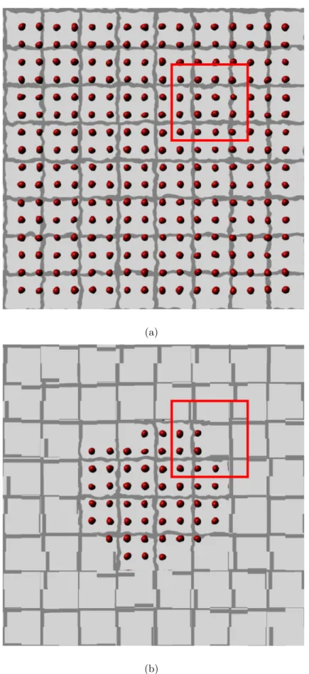
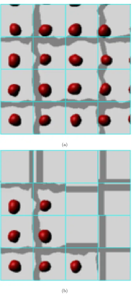
Hermann grid illusion is a very famous optic illusion, which consists of several black rectangles laid on a white background like city blocks as shown in Fig.C.7(a). We can observe a gray spot appears at crossroads. It’s said that this illusion is caused by lateral inhibition.

We choose a kernel size larger than that described in §C.3.2, because this optic illusion occurs on where retinal eccentricity ratio is large. The filtered image is shown in Fig.C.7(b). Fig.C.8 shows three dimensional views of the gradients of Fig.C.7(a) and (b). A basin of the brightness appears at the crossroad. This means that our filters can approximate the sensory properties of human visual system.

C.4.3

Direction Boards

(a) (b)

図 C.7: An approximation result of Hermann grid. (a) An original image, (b) Lateral inhibition filtering applied image

board is 2.2 meters height and 2.8 meters width, (2) distance of sight is 30 meters and 100 meters away from the board, and (3) eyesight of viewers is 20/20, 20/30, 20/60. We apply our filters to the board image, and generate the images as shown in Fig.C.9. These simulation results verify that our filters can generate appropriate blurred images corresponding to eyesight, and visual angle adjustment including visual contrast due to lateral inhibition phenomena.

C.5

Concluding Remarks

In this paper, we proposed a visual simulation method of viewers’ eyesight based on image filtering approach. Considering the properties of human visual system, we measured and found several appropriate parameters for our filters experimentally, and confirmed their validity.

• We verified our filters can simulate arbitrary eyesight by the experiments on

(a)

characters of Snellen chart which test viewers’ eyesight are almost equal from the point of view of characters recognition capability.

• Our method succeeded in simulating one of the most famous optic illusions,

Hermann grid illusion, by applying our filters considering the lateral inhibition phenomenon.

• We simulated visual appearance of direction boards were at 30 meters and 100 meters away from the board, and viewers’ eyesight varied from 20/20, 20/30 to

20/60. Simulated appearance of the direction board also satisfied that visual angle adjustment as well as blurred images corresponding to eyesight.

simulated Distance of sight

eyesight 30 meters 100 meters

20/20

20/30

20/60

付 録

_D

研究業績一覧

D.1

査読付き論文

( Journal Papers )

[JP-1] 金澤功尚, 田邉竜馬, 森谷友昭, 高橋時市郎: “オブジェクトの形状を考慮

した錆によるエイジング画像シミュレーション”, 画像電子学会誌, Vol.46, No.4, pp.547-558, (2017)

[JP-2] Katsuhisa Kanazawa, Yuma Sakato, Tokiichiro Takahashi: “Pencil

Trac-ing Mirage Fast Generation Method of Mirage based on Paraxial Ap-proximation Theory”, ITE Transactions on Media Technology and Appli-cations, Vol.1, No.4, pp.307-316, (2013)

[JP-3] Katsuhisa Kanazawa, Yasuko Nakano, Tomoaki Moriya, Tokiichiro

Taka-hashi: “Visual Appearance Simulation Method for Exhibited Objects Considering Viewer ’s Eyesight and Lateral Inhibition”, 画像電子学会 誌, Vol.40, No.1, pp.151-158 (2011)

D.2

国際会議

( International Conferences )

いずれも査読有り

[IC-1] Katsuhisa Kanazawa, Ryoma Tanabe, Tomoaki Moriya, Tokiichiro

[IC-2] Katsuhisa Kanazawa, Tomoaki Moriya, Tokiitiro Takahashi: “Video-based

Mirage for Extended Pencil Tracing”, 2015 Joint Conference of IFMIA and IWAIT, Tainan, Taiwan (2015)

[IC-3] Katsuhisa Kanazawa, Yuma Sakato, Tokiichiro Takahashi: “Pencil

Trac-ing Mirage: Principle and its Evaluation”, ACM SIGGRAPH 2013 Tech-nical Talks, Anaheim, USA (2013)

[IC-4] Katsuhisa Kanazawa, Yuma Sakato, Tokiichiro Takahashi: “Pencil

Trac-ing Mirage: Principle and its Evaluation”, ACM SIGGRAPH 2013 Tech-nical Posters, Anaheim, USA (2013)

[IC-5] Katsuhisa Kanazawa, Yuma Sakato, Tokiichiro Takahashi: “Pencil

Trac-ing Mirage Fast Generation Method of Mirage based on Paraxial Approx-imation Theory “, International Workshop on Advanced Image Technol-ogy (IWAIT2013), Nagoya, Japan (2013)

[IC-6] Katsuhisa Kanazawa, Takafumi Arai, Tomoaki Moriya, Tokiikichiro

Taka-hashi: “A Walking Motion Morphing Method Based on Statistical Data of the Elderly”, ACM SIGGRAPH 2011 Technical Posters, Vancouver, Canada (2011)

[IC-7] Katsuhisa Kanazawa, Kazushi Urabe, Tokiichiro Takahashi: “An Image

Query-based Approach for Urban Modeling”, ACM SIGGRAPH ASIA 2010 Technical Sketches, Seoul, Korea (2010)

[IC-8] Katsuhisa Kanazawa, Yasuko Nakano, Tomoaki Moriya, Tokiichiro

技術フォーラム) 講演論文集, I-045 (2010)

[DC-7] 浦辺一志，金澤功尚, 森谷友昭，高橋時市郎: “ビル群画像からの類似した

街並みのモデリング法”, Visual Computing / グラフィクスと CAD 合同 シンポジウム 2010 (2010)

[DC-8] 中野泰子，金澤功尚，高橋時市郎: “視力と側抑制効果を考慮した展示物