Skill sorting and production chains : evidence
from India
著者
Asuyama Yoko
権利
Copyrights 日本貿易振興機構(ジェトロ)アジア
経済研究所 / Institute of Developing
Economies, Japan External Trade Organization
(IDE-JETRO) http://www.ide.go.jp
journal or
publication title
IDE Discussion Paper
volume
545
year
2015-11-01
INSTITUTE OF DEVELOPING ECONOMIES
IDE Discussion Papers are preliminary materials circulated to stimulate discussions and critical comments
Keywords: India, Input quality, Production chains, Return to skill, Skill sorting, Skill wage premium
JEL classification: I25, I26, J24, J31, L23, O15
IDE DISCUSSION PAPER No. 545
Skill Sorting and Production Chains:
Evidence from India
Yoko Asuyama*
November 2015
Abstract
This study proposes a new mechanism that explains skill-sorting patterns and skill wage differentials across industries based on the length of the industry’s production chain. A simple simultaneous production model shows that when the quality of intermediate inputs deteriorates rapidly along the production chains, high-skilled individuals choose to work in industries with shorter production chains because of higher returns to skill. I empirically confirm this skill-sorting pattern and these inter-industry skill wage differentials in India, where the quality of intermediate inputs is likely to degrade rapidly because of the high number of unskilled laborers, poor infrastructure, and less-advantaged technology. The results remain robust even when considering selection bias, alternative reasons for inter-industry skill wage differentials, and a different period. The results of this study have important implications when considering countries’ industrial development patterns.
The Institute of Developing Economies (IDE) is a semigovernmental, nonpartisan, nonprofit research institute, founded in 1958. The Institute merged with the Japan External Trade Organization (JETRO) on July 1, 1998. The Institute conducts basic and comprehensive studies on economic and related affairs in all developing countries and regions, including Asia, the Middle East, Africa, Latin America, Oceania, and Eastern Europe.
The views expressed in this publication are those of the author(s). Publication does not imply endorsement by the Institute of Developing Economies of any of the views expressed within.
INSTITUTE OF DEVELOPING ECONOMIES (IDE), JETRO 3-2-2, WAKABA,MIHAMA-KU,CHIBA-SHI
CHIBA 261-8545, JAPAN
©2015 by Institute of Developing Economies, JETRO
Skill Sorting and Production Chains: Evidence from India
Yoko Asuyama
*†Abstract
This study proposes a new mechanism that explains skill-sorting patterns and skill wage differentials across industries based on the length of the industry’s production chain. A simple simultaneous production model shows that when the quality of intermediate inputs deteriorates rapidly along the production chains, high-skilled individuals choose to work in industries with shorter production chains because of higher returns to skill. I empirically confirm this skill-sorting pattern and these inter-industry skill wage differentials in India, where the quality of intermediate inputs is likely to degrade rapidly because of the high number of unskilled laborers, poor infrastructure, and less-advantaged technology. The results remain robust even when considering selection bias, alternative reasons for inter-industry skill wage differentials, and a different period. The results of this study have important implications when considering countries’ industrial development patterns.
JEL Classification: I25, I26, J24, J31, L23, O15
Keywords: India, Input quality, Production chains, Return to skill, Skill sorting, Skill wage premium
.
*
Institute of Developing Economies, Japan External Trade Organization (IDE-JETRO), Wakaba 3-2-2, Mihamaku, Chiba, 261-8545, Japan. E-mail: [email protected].
†
I thank Yuji Genda, Hideaki Goto, Mizuki Harizuka, Masami Ishida, Satoshi Inomata, Md. Humayun Kabir, Tomohiro Machikita, Mayumi Murayama, Mari Nakamura, Hiroshi Sasaki, Jeffrey M. Wooldridge, and all the internal seminar participants at the Institute of Developing Economies, Japan External Trade Organization (IDE-JETRO), and the University of Tokyo. This paper is the research output of the IDE-JETRO’s FY2014–15 research project entitled “Transition from School to Work: Linkage of Education and Employment in India.” I am grateful for the funding support from the IDE-JETRO
1. Introduction
It is widely known that India’s recent economic growth has been fueled by
service sectors such as business services (including software and information
technology (IT)-enabled services), communications, and banking. More-traditional
services, including hotels and restaurants, education, health, and trade and transport,
have also undergone rapid growth (Eichengreen and Gupta, 2011). Since 1999 (up to
2014), service industries’ share of the gross domestic product (GDP) has exceeded 50%
in India (World Bank, 2015). This share seems large if India’s development stage is
considered. India’s share of services in the GDP outweighed its predicted value for
India’s income by 6 percentage points on average from 1999 to 2014.1
One possible cause for India’s service-led growth is its skill-sorting pattern. As
Kamath (2011) and Sohoni and Kathuria (2014) showed, many highly talented
graduates who studied engineering at the Indian Institutes of Technology (IIT), the most
distinguished institutions of higher education in India, go on to choose non-engineering
occupations, such as IT, finance, and consultancy services. For example, only 33% of
students at IIT Bombay took engineering jobs in 2013 (Sohoni and Kathuria, 2014).
Those highly intelligent students should foster India’s manufacturing industries, but
they do not; instead, they contribute to strengthening the competitiveness of India’s
service sector. This skill-sorting trend operates across all of India too. Because of
individual-level skill sorting, the workforce’s educational level tends to be higher in
many service industries. In Figure 1, industries are sorted by the estimated number of
completed years of education averaged over an industry’s male regular wage/salaried
(RWS) workers. The average education level of an industry’s workforce falls in moving
1
India’s predicted value for the share of services in GDP is computed based on the cross-country OLS regression of share of services in GDP on a quartic polynomial in log of GDP per capita for the period 1960–2014 over 215 economies. Data are extracted from the World Bank (2015). The service industries correspond to divisions 50–99 of the International Standard Industrial Classification (ISIC), revision 3. Note that they do not include construction, electricity, water, and gas, which are classified as services in my study.
from left to right across the graph. Therefore, it is clear from the graph that many
service industries, such as insurance (industry number 53), education and research (54),
finance (banking, etc.; 52), medical and health services (55), post and
telecommunication (51), public administration and defense (57), railway transport (49),
electricity (44), and other services (56), are successful in attracting relatively
higher-educated workers.
Why does this skill-sorting pattern occur? Kamath (2011) and Sohoni and
Kathuria (2014) gave wage differentials as one possible cause. However, why are wages
lower for engineering jobs compared to other service-sector jobs, such as business
services and banking?
This study offers one possible answer to this question. I hypothesize that
India’s skill-sorting patterns and skill wage differentials are a result of interactions
among India’s unequal skill distribution, low input quality, and variations in industries’
production chain lengths. First, producing manufacturing goods tends to require more
intermediate inputs than needed to produce service goods. In other words,
manufacturing industries tend to form longer production chains than service industries.
This tendency is confirmed from the line graph in Figure 1 (or Figure 3 in Section 6).
Second, similar to the O-ring theory by Kremer (1993), the quality of final good
deteriorates more as more intermediate inputs are involved as a result of increased
defect rates. For example, if the probability of a malfunction in each part is 1%, then
that of a product composed of two units of the part becomes 1.99%
(=1-0.99*0.99)*100). As will be discussed below, the magnitude of such quality
deterioration is likely to be larger in a country such as India. In this case, wages in
manufacturing industries that require many intermediate inputs are dragged down
significantly because of substantial quality deterioration compared to wages in service
industries. Consequently, high-skilled individuals choose not to work in manufacturing
in service industries.
The quality deterioration concomitant with an increase in intermediate inputs is
expected to be much more severe in developing countries such as India, which are
characterized by a large pool of unskilled labor, poor infrastructure (e.g., unstable
electricity supply and bumpy roads), and less-advanced technology. These factors all
contribute to low-quality intermediate inputs and much higher defect rates when many
inputs are combined. As of 2009–2010, 41% of India’s working population are either
illiterate or literate, but they have either never received formal education or failed to
complete primary education (based on weekly status computed from NSSO (2009–
2010)). According to the 2014–2015 Global Competitiveness Report published by the
World Economic Forum, India ranks 103rd in terms of quality of electricity supply and
76th in terms of quality of roads among the 144 countries included in the report (World
Economic Forum, 2014). In addition, India’s rank in terms of local supplier quality,
availability of latest technologies, and firm-level technology absorption is 78th, 110th,
and 102nd, respectively, indicating the generally low quality of intermediate inputs in
India. Although it is difficult to directly measure the quality of intermediate inputs in
India, some examples can be offered here. For example, UNIDO (2010: p.7) cites a
survey conducted by A.T. Kearny, who found that defect rates in the Indian auto
component industry are in the range of 1000–2000 parts-per-million (ppm), whereas
those of Japanese average around 100–200 ppm. World Bank (2004: p.52) also
mentioned the low quality and quality inconsistency of India’s textile and clothing
products, which is likely to be a consequence of a fragmented production process spread
over many small-scale units.
This study contributes to the literature in two main ways. First, it proposes a
new mechanism that explains India’s skill-sorting pattern, which is, in turn, likely to
contribute to India’s service-led growth. Second, this study theoretically and empirically
differentials across industries based on the length of an industry’s production chains (or
the amount of necessary intermediate inputs used to produce an industry’s output). I
present a simple model to show that when the quality of intermediate inputs deteriorates
rapidly, exceeding the increasing speed of marginal revenue of skill, workers’ skill is
negatively associated with the length of an industry’s production chains. In other words,
higher-skilled individuals choose to work in industries with shorter production chains.
In this study, I call this skill-sorting pattern negative sorting, and the opposite pattern is
called positive sorting. Negative (positive) sorting occurs because wage returns to skill
are higher in industries with shorter (longer) production chains. Using India’s data for
year 1999, I empirically confirm the existence of negative sorting because of seeking a
higher return to skill in India. The results remain robust even when correcting for
possible selection bias, controlling for alternative reasons for inter-industry skill wage
differentials, and examining the 2009 data alone.
The rest of the paper is organized as follows. Section 2 overviews related
studies and the ways in which this study contributes to the literature. Section 3 presents
a simple simultaneous production model in which skill-sorting patterns depend on the
length of industry production chains and intermediate input quality. Section 4 explains
the empirical strategy. Section 5 describes the data sources and the construction of key
variables. Section 6 presents the main estimation results for India in 1999. Section 7
provides robustness checks, and Section 8 concludes.
2. Related Literature and Contribution of This Study
First, this study is closely related to studies that examine how high-skilled
workers are matched with other workers or intermediate inputs (Kremer 1993; Lucas
1978; Murphy, Shleifer, and Vishny 1991; Rosen 1982; Sampson 2013). All studies are
Moreover, most studies present models in which high-skilled workers are matched with
larger amounts of labor or intermediate inputs. For instance, most talented persons
produce products that require more tasks (and thus, require more high-skilled workers)
or work at later stages of sequential production (Kremer 1993), manage firms with
larger numbers of employees (Lucas 1978; Murphy, Shleifer, and Vishny 1991; Rosen
1982), or work with larger amounts of high-quality intermediate inputs (Sampson 2013).
My study shares common features with Kremer (1993) in terms of introducing quality
deterioration as the number of inputs increases and with Sampson (2013) in terms of
examining the matching of workers’ skills with the quantity and quality of intermediate
inputs. However, my study shows that an opposite matching pattern is possible:
high-skilled workers can work with a smaller amount of intermediate inputs when the
quality of intermediate inputs deteriorates substantially along the production chains.
Second, in terms of results, my study also shares certain features with
Grossman (2004) and Asuyama and Goto (2015). Grossman (2004) built a two-sector
model to show that most talented individuals choose the so-called “software” sector, in
which they can work alone and get paid according to their own productivity. They are
disinclined to work in a team production sector (“automobile” sector) in which the
wages of high-skilled workers are dragged down by low-skilled team members because
of imperfect labor contracts. I differ from Grossman (2004) in terms of introducing
intermediate inputs, building a different multi-sector model, and providing an empirical
analysis. Asuyama and Goto (2015) theoretically showed that high-skilled individuals
choose to work at earlier production stages when the quality of intermediate input
deteriorates rapidly or improves slowly with each production stage. Based on
cross-country industry panel data, they also empirically confirmed their model’s
prediction. However, their model is based on sequential production, while mine
considers simultaneous production. In addition, their data is less fine compared to mine.
In addition, their classifications of industry and skill are much broader.2 They do not
provide any analysis on inter-industry skill wage differentials. Focusing on one country
(i.e., India), I examine skill-sorting patterns and inter-industry skill wage differentials
more rigorously in this paper.
Finally, this study is also related to studies based on Roy’s model (Roy, 1951),
which explains skill wage differentials and skill allocation across sectors. Different
wage returns to observed or unobserved skills across sectors, such as industries or
occupations, have been found in several empirical studies (Gibbons, Katz, Lemieux, and
Parent, 2005; Heckman and Scheinkman, 1987; Keane and Wolpin, 1997; Pavcnik,
Blom, Goldberg, and Schady, 2004). Pavcnik et al. (2004) speculated that returns to
skill differ across sectors because (1) labor mobility, (2) the ability to bargain over
wages, and (3) monitoring costs and the necessity of paying efficiency wages all differ
between high- and low-skilled workers. Roy’s self-selection framework offers another
explanation. In this framework, workers are endowed with multiple sector-specific skills
and can have only one job. In this situation, workers self-select into jobs based on their
comparative advantage. That is, they choose occupations that offer higher returns to a
skill with which they are relatively well endowed. Autor and Handel (2013) and
Yamaguchi (2012) obtained some empirical support for this mechanism. Most Roy-type
studies state that skills are differently rewarded across sectors because skill
requirements vary among them. My study offers an alternative mechanism, that is,
returns to skill can vary among sectors because of differences in production chain
lengths.
3. Model
2
The number of industries is around 35. In addition, only three skill categories based on education level are available.
Based on a simultaneous production model, this section analyzes how
skill-sorting patterns are affected by intermediate input quality and production chain
length. My model builds upon the O-ring theory by Kremer (1993) in terms of
introducing quality deterioration with an increase in inputs and upon Sampson (2013) in
terms of introducing the quantity and quality of intermediate inputs.
Consider a perfectly competitive economy with multiple industries. The output
of a certain industry is produced by many identical production units, each of which
comprises one individual with a skill (or productivity) of θ ∈[0,1] who is working on n units of intermediate inputs. There exists only one type of intermediate input, which is the composite of various inputs.3 Each industry is only distinguished by n (amount of
necessary intermediate inputs), which I call the industry’s length of production chains.
As with Sampson (2013), because of the zero-profit condition in a perfectly
competitive market, each worker’s wage equals the profit of his/her production unit,
which is equal to revenue minus the cost of intermediate inputs. Then, by solving the
wage maximization problem below, an individual will choose to work in industry n*
where he/she can receive the highest wage:
MaxW n q Q q nV n nq n − = ( , ) ( , ) ) , , (θ θ , (3.1)
where W(θ,n,q) is the wage of a worker with skill θ if he/she chooses industry n and works on n units of intermediate inputs of quality q. q∈(0,1] is the quality of one unit of intermediate input, which is assumed to be exogenously determined by various
factors, including levels of human capital, technology, and infrastructure of the economy.
) , ( nq
Q stands for the quality of aggregated intermediate inputs when n intermediate inputs with quality q are used to produce output. Qq >0 is assumed.4 Importantly, and
3
Here, the proportion of various inputs is assumed to be the same among composite inputs, although this is not a realistic assumption. Incorporating heterogeneity of inputs is left for future research.
4
The notation “Yx” stands for partial derivative of Y with respect to x.
similar to the O-ring theory by Kremer (1993), I assume that Q is decreasing in n
(Qn <0) because the possibility of defects increases as more inputs are involved. For example, consider the quality of a car. If the failure rate of brakes and engines are 1%
each, the probability of a car that incorporates both parts failing to work properly
becomes 1.99% (= [1−0.99*0.99]*100). In terms of defect rate, the car’s overall quality (final output quality) becomes worse than the quality of each part. Even if the quality of
each input is perfect (q = 1), a negative Q can still occur if the assembly process n itself entails quality deterioration that becomes more severe with an increase in inputs.
Similarly to Kremer (1993), output price and quantity are combined in one function,
) , ( n
V θ , which is the value of output achieved if intermediate input quality exerts no influence. I assume Vθ >0, Vn >0 and that both Q and V are twice-continuously differentiable. QV is the total revenue of the production unit. The price of one unit of
intermediate input with perfect quality (that is, q = 1) is standardized to one. Thus, the
cost of intermediate inputs is expressed by nq. Finally, I assume Qnn <0 and 0
<
nn
V .5
The first-order condition for the worker’s maximization problem becomes
Wn =QnV +QVn −q=0. (3.2) Then, by the implicit function theorem,
n n nn nn n n V Q QV V Q QV V Q d dn 2 * + + + − = θ θ θ . (3.3)
Because of the assumptions of Qnn <0 , Vnn <0 , Qn <0 , and Vn >0 , the denominator, which is the left-hand side of the second-order condition, is negative. If
θ
d
dn /* is negative, it implies that if an individual’s skill level is higher, the amount of intermediate inputs he/she chooses to work with is lower (i.e., the industry’s length of
production chains is shorter). Such negative sorting (dn*/dθ <0) occurs only when
5
These two assumptions are not necessary but are sufficient conditions for the second-order condition to be satisfied.
0 < + θ θ n nV QV Q , or equivalently Q Q V Vn n − < θ θ
. (3.4: negative sorting condition)
By assumption, Qn <0, Vθ >0, and Q > 0. The sign of Vθncan be either positive (when V is supermodular in workers’ skill and amount of intermediate inputs) or
negative (when V is submodular). When V is supermodular (Vθn >0), this condition shows that when the speed of quality deterioration along the production chains exceeds
the increasing speed of marginal revenue of workers’ skill (V ), negative sorting occurs. θ On the other hand, if the magnitude of quality deterioration is not sufficiently large,
positive sorting occurs. When V is submodular (Vθn <0), equation (3.4) always holds regardless of the degree of quality deterioration. Even when no quality deterioration
occurs (Qn =0), negative sorting can occur if V is submodular because the marginal revenue of a worker’s skill falls as the production chain lengthens. Finally, it should be
noted that regardless of the sign on Vθn, high-skilled individuals choose smaller-n industries because these industries offer the highest wages. For low-skilled individuals,
however, a larger-n industry offers higher rewards. In this sense, returns to skill (or skill
wage premiums) are larger in industries with shorter production chains, when negative
sorting occurs under condition (3.4).
4. Empirical Strategy
This section tests (1) whether negative sorting occurs in India and (2) whether
the returns to skill are larger in industries with shorter production chains. The model in
the previous section indicates that when sorting depends on input quality (that is, when
V is supermodular), negative sorting is more likely to be observed in developing countries such as India, where it can be expected that the input quality will fall rapidly
as a result of many unskilled workers, low technology, and poor infrastructure.6 In
addition, as the skill distribution throughout the economy becomes more unequal, this
skill-sorting trend emerges more sharply. In this sense, India is one of the most
appropriate fields to examine skill-sorting patterns given its relatively large number of
highly educated population as well as its large pool of unskilled workers. In 2009−2010, the proportion of workers who had received no schooling or failed to complete primary
education was 41% (as mentioned above), compared to the 15% who had completed
secondary education (computed based on NSSO (2009–2010)).
If V is submodular, negative sorting occurs regardless of the input quality in the
economy. However, this submodular-V case can be excluded using the evidence from
Asuyama and Goto (2015), which shares a similar hypothesis to that of this paper.
Based on cross-country industry panel data, they empirically show that the economy’s
skill-sorting pattern depends on the input quality in the economy. Their results show that
negative sorting occurs only in economies in which the rate of change in intermediate
input quality along production chains is small (either quality deteriorates rapidly or
improves slowly). Regardless of specifications, their results imply that negative sorting
occurs in India, where input quality degrades rapidly (or improves slowly). However,
the data from Asuyama and Goto (2015) is less fine compared to the data in the current
paper (see Section 2). Thus, I examine India’s skill-sorting pattern more rigorously in
this paper. I also examine whether skill sorting is affected not only by production chain
length but also by other supplemental quality indicators of intermediate inputs in order
to test whether India’s skill-sorting pattern depends on input quality.
6
As explained in the car example in Section 3, it is natural to expect that low quality of an intermediate input (low q) leads to a large negative value of Qn and that low q is caused by unskilled labor, low technology, and poor infrastructure, such as unstable electricity supply and bumpy roads.
4.1 Skill-Sorting Regression
To test whether negative sorting is observed in India, the following three
equations are estimated using weighed least squares (WLS). The weight used is the
survey weight of the dataset (equation (4.1)), the employment size of each industry
(equation (4.2)), and the employment share of each industry averaged over the two
periods (equation (4.3)), respectively:
ChainLijt =a1t +β1tSkillijt +γ1tXijt +δ1tChainL_sfamilyijt +ε1ijt, (4.1) jt jt t jt t jt t t jt ChainL ChainQ Z Skill =a2 +β2 +γ2 +δ2 +ε2 , (4.2) jt j t jt jt jt jt ChainL ChainQ Z F F Skill =a3+β3 +γ3 +δ3 + + +ε3 , (4.3)
where subscripts i, j, and t denote worker, industry, and time period (mainly 1999 and
2009 as a robustness check), respectively. In every equation, ε stands for the error term. In equation (4.1), ChainLijt measures the length of domestic production chains
of industry j with which individual i is affiliated. Skillijt stands for i’s skill level.
it
X denotes a vector of individual characteristics, which includes estimated years of work experience and its square, dummies for being a Muslim, social groups, household
head, marriage status, residence in rural area, and Indian states in which an individual
lives.7 ChainL _sfamilyijt is the average ChainLijt of other family members of the
same gender. This is included because in India, an individual’s job choice is assumed to
be substantially affected by the jobs of same-gender family members.8 Equation (4.1) is
estimated separately for each period and at the individual level. If β1t <0 is observed, it indicates negative sorting; that is, high-skilled individuals choose industries with
shorter production chains.
Because industry characteristics other than the length of production chains
7
When the elements constructing my skill index (see Section 5.2.1) include work experience (i.e., in cases of SK2 and SK3), experience and its square are not controlled for. Such a treatment also applies when testing inter-industry skill wage premium later.
8
I also experiment with controlling for the average ChainL of other same-gender workers in the same district in addition to ChainL_sfamily, but the main results do not change.
cannot be controlled for in equation (4.1), equation (4.2) is also estimated separately for
each period but at the industry level.9 Skilljt and ChainLjt stand for the average skill
level of workers and the length of domestic production chains for industry j at time t,
respectively. If negative sorting occurs, workers’ skill level should be higher in
industries with shorter production chains. In this case, β2t should be negative. jt
ChainQ represents a vector of supplemental quality indicators of intermediate
inputs that are not captured by ChainLjt. It includes an industry’s dependence on
imported inputs (ChainQ _Importjt) and the skill level embodied in inputs from other
industries (ChainQ _Skilljt). ChainQjt is controlled for because in reality, the input
composition differs across industries. Consequently, the size of quality deterioration is
determined by not only production chain length but also input composition and quality.
It is expected that the quality of imported inputs is higher than that of domestic inputs.
In addition, input quality can be measured by the skill level of workers who produce
said inputs. A statistically significant value for γ2t implies that a skill-sorting pattern depends on input quality (supermodular-V case). A positive value for γ2t is expected because when comparing industries with the same ChainLjt, input quality deterioration
can be expected to be smaller in a higher-ChainQjt industry, which consequently
attracts more skilled workers.
jt
Z denotes a vector of industry characteristics. It includes degrees of imports
and exports of final goods. It also includes employment ratios of small firms, which
approximate an industry’s degree of informality.
Finally, industry-level skill-sorting equation (4.3) is estimated by pooling
two-year samples and adding time and industry fixed effects (F and t Fj, respectively).
j
F controls for all time-invariant industry characteristics, some of which are not
9
Here, I do not aim to identify causality but try to confirm the association between worker’s skill level and production chain length. Thus, either Skill or ChainL can become the dependent or independent variable.
controlled for in equation (4.2). Again, a negative β3 and positive γ3 can be expected.
4.2 Skill Wage Premium Regression
To test whether the return to skill is larger in industries with shorter production
chains, the following augmented Mincer-type wage equation (Mincer, 1974) is
estimated by WLS with the survey weight:
ijt ijt t ijt ijt t ijt ijt t t
ijt Skill ChainL Skill ChainQ Skill Z
Wage * * * ln =a4 +β4 +γ4 +δ4 ijt j ijt t ijt tSkill 4 X F 4 4 l ε η + + + + , (4.4)
where lnWageijtdenotes the logarithm of a worker’s wages in industry j at time t. If
t 4
β , the coefficient of the interaction term between Skillijtand ChainLijt is negative, it indicates that returns to skill are higher in industries with shorter production chains.
As in the skill-sorting regressions, supplemental quality indicators of the chain
(ChainQijt) are also controlled for. A positiveγ4t is expected because it is expected that
input quality deteriorates with a decrease in ChainQijt . Similar to the effect of
ijt
ChainL , this effect of quality deterioration can lead to a lower return to skill.
To control for other reasons causing inter-industry skill wage differentials, a
vector Zijtis also interacted with Skillijt. It contains individual characteristics, such as
union affiliation, employment nature (permanent or temporary), and affiliation with
public and small firms. These factors are included because it can be expected that a skill
wage premium applying to union members or public-sector workers would be smaller
because the effect of market forces on the wage-setting mechanism might be weaker in
these sectors. Based on empirical evidence from India (Azam, 2012; Dutta, 2006), it can
also be expected that the skill wage premium is lower in informal sectors characterized
by temporary employment or small firm size.
it
X is a vector of individual characteristics such as those included in equation (4.1) as well as occupation, union affiliation, employment nature, social security status,
and affiliation with a public and small firm.10 Controlling for these variables is
particularly important in India, where a large informal sector exists. Industry affiliation
dummies (Fj) are also included. Fj absorbs the industry-wage premium that is
common for all workers regardless of their skill level. Finally, ε denotes the error 4ijt term.
The above identification strategy is possible because individuals with the same
skill level choose different industries and receive different wages in India’s dataset. This
fact can be explained by the model developed by Dahl (2002), in which individuals
maximize their utility, which is a function of earnings and tastes.11 Thus, in reality,
wages and individuals’ preferences regarding job characteristics affect their industry
choice. As a result, perfect negative sorting is not observed, and inter-industry (or more
precisely, inter-ChainL) skill wage differentials can be identified.
5. Data
5.1 Main Data Sources and Sample Used
Data on individual-level variables, including wages, skill level, and other
characteristics, as well as several industry-level variables, such as workers’ skill level of
industry, are primarily constructed from the unit-level data of the Employment and
Unemployment schedules of the National Sample Survey (NSS). As Kijima (2006)
states, the Employment and Unemployment schedule of the NSS is the only survey that
collects information on individual’s earnings, employment status, and other
characteristics for all of India through a stratified random sampling procedure.
10
Similar to the treatment in footnote 7, if the skill index is constructed from education, experience, and occupational information (i.e., in case of SK3), experience and occupations are not controlled for when estimating equation (4.4).
11
Dahl (2002) theoretically and empirically examined individuals’ patterns of self-selection and the difference in return to education across U.S. states.
Industry-level data, including the length of production chains, dependence on
imported inputs, and import or export ratio, are constructed from the input-output (IO)
tables for India.
I primarily examine the matched data on the 55th round of NSS data conducted
in 1999–2000 and the 1998–1999 IO table (NSSO, 1999-2000; CSO, 1998-99). I call
this period 1999. Year 2009 data, which is the matched data on the 2009–2010 (66th
round) NSS and the 2007–2008 IO table (NSSO, 2009-2010; CSO, 2007-08), is also
examined in the robustness analysis and used in the industry-panel skill-sorting
regression (equation (4.3)). There are several reasons for primarily analyzing the 1999
data. First, the NSS sample size is much larger in this period, and consequently, the
most finely grained industry classifications can be achieved.12 Second, before this round,
the NSS did not collect some important information, such as firm size and social
security status. Third, after this round, it is not possible to construct accurate skill
indices that incorporate occupational information because NSS occupational
classifications become much broader. Finally, both ChainL and ChainQ become less
accurate in subsequent years.13
There are 115 sectors in the 1998–1999 IO table. I match these sectors with the
NSS’s five-digit industry codes as closely as possible based on the descriptions of both
sectors and industries. I also ensure that there is a sufficient number of observations
(around 100 sample workers) with non-missing wage information for each industry
because the within-industry wage gaps between skill groups is estimated in equation
(4.4). As a result, 57 industries are created.14 The concordance table on industry
12
The numbers of households and individuals covered by the NSS are 115,409 and 564,740 (1993–1994), 165,244 and 819,013 (1999–2000), 124,680 and 602,833 (2004–2005), and 100,957 and 459,784 (2009–2010), respectively.
13
This is because the construction of these two indices involves estimation based on the 1993– 1994 IO table, for which the industry classification is the same as the 1998–1999 IO table but different from the 2007–2008 IO table (see Sections 5.2.2 and 5.2.3).
14
When year 2009 data is examined as a robustness check in Section 7.3, 54 industries are created as a result of the same procedure. For the details of these 54 industry classifications, see
classification between IO tables and the NSS is provided in Appendix Table B.3(a).
I restrict the estimation sample to male, prime-age (15–65 years old), regular
wage/salaried (RWS) employees who have worked full time and are not currently
attending an educational institution. Following Kijima (2006), full-time workers are
defined as those who have worked at least five days at their main economic activity
during the reference week.15 Because the actual hours worked are not asked in the NSS,
wages are defined as the weekly wage and salary earnings (either in cash or in kind,
including bonus and perquisites) for the main economic activity.
5.2 Construction of Key Variables
This subsection describes how I construct key variables, namely Skillijt,
jt
ChainL , and ChainQjt. A brief description of other variables and the summary
statistics are presented in Appendix A.
5.2.1 Skill: Workers’ Skill
Workers’ skill (Skillijt) is measured by the following three (or four) indices: Skill index 1 (SK1), which equals estimated years of education: Measuring
individuals’ skills by their levels of educational attainment is the most conventional
method used in the labor and macroeconomics literature (Ingram and Neumann,
2006: p.37). Seven educational levels (illiterate; literate without formal schooling or
Appendix Table B.3(b).
15
Wages, RWS working status, number of days worked, and industry and occupation affiliations are based on the status during the reference week. However, other individual characteristics, such as union affiliation, employment nature, social security status, and affiliation with a public firm and small firm, are only available for so-called “usual status,” which is based on a reference period of one year. Thus, when controlling for these characteristics, I restrict the sample to individuals whose RWS working status, five-digit industry code, and three-digit occupation code are the same between weekly and usual (yearly) statuses. I also restrict this sample by only focusing on individuals who explicitly claim that they had no months without work during the reference year. Under this restriction, I assume that individuals’ jobs based on weekly and yearly status are the same.
literate but have not completed primary education; primary; middle; secondary;
higher secondary; graduate and above) can be identified in NSS 1999–2000. The
years of education are estimated from these seven categories by allocating the
corresponding number of years of schooling to each level respectively (0, 2.5, 5, 8,
10, 12, and 15 years).
Skill index 2 (SK2), which is constructed from education and experience: An alternative skill index is constructed following Gibbons et al. (2005: p.698). First, a
logarithm of wages is regressed on education category dummies, X , in equation it (4.1) (or equation (4.4), depending on the specification of the regressions
considered) and industry affiliation dummies.16 Then, skill index 2 (SK2) is
estimated by predicting the wage of each worker based solely on the worker’s
education and experience. Because the numbers of years of work experience are not
available in NSS data, they are estimated by subtracting [estimated years of
education plus 5] from age, following Kijima (2006). Finally, this skill index is
normalized to have a zero mean.
Skill index 3 (SK3(1) and SK3(2)), which is constructed from education, experience, and task content of occupation: Skill index 3 (SK3) is computed similarly as the predicted wage based on education, experience, and task content
measure of occupations.17 Autor and Handel (2013) showed that workers self-select
into occupations that offer high returns to tasks in which they are relatively well
endowed. Thus, I assume that occupation task content can be used as a proxy for a
16
When examining SK2 in skill-sorting regression, Xitof equation (4.1) is used. In case of a skill wage premium regression, Xitof equation (4.1) is used when occupations, union affiliation, employment nature, social security status, and affiliation with a public and/or small firm are not controlled for in the regression. When these variables are controlled for in the skill wage premium regression, Xitof equation (4.4) is used.
17
Before prediction, the logarithm of wages is regressed on education category dummies, task content measures of occupations, Xitin equation (4.1) (or equation (4.4) ) without occupation dummies, and industry affiliation dummies.
worker’s skill in conducting these tasks. I experiment with two task content
measures of occupation. The first measurement used to construct SK3(1) is
cognitive and motor task complexity of occupations, which was extracted from
Yamaguchi (2012). The second measurement used for SK3(2) is routine, abstract,
and manual task intensity of occupations, which was extracted from Autor and
Dorn (2013) and Dorn (2009). Because both measurements are constructed based
on the task content of occupations in the United States (U.S.) around 1991 or 1977,
they might be crude measures for the task content of India’s occupations. However,
as long as some commonality can be expected between occupation-specific skill
requirements in the U.S. and India, SK3 can serve as an appropriate proxy for
ijt
Skill . Based on occupation content, I match occupation codes between India and
the U.S. as closely as possible (Appendix Table B.4(b)). Then, occupation-specific
task content measures for the U.S. are assigned to each occupation in India.
Because the occupation codes in the 2009–2010 NSS are much broader than those
in the 1999–2000 NSS, SK3 is constructed only for 1999.
5.2.2 ChainL: Length of Production Chains
The length of production chains of industry j (ChainLjt) is computed in a
manner similar to that used in Asuyama (2012). In general, ChainLjt is the column
sum of the Leontief inverse coefficient of industry j computed from the aggregated
57×57 sector IO table as follows:
∑
=k kjt
jt leon
ChainL , (5.1)
where leonkjt is the (k, j)th entry of the Leontief inverse coefficient matrix, L.18
jt
ChainL measures the amount of domestic intermediate inputs that industry j requires,
18 1
) ( − − = I Ad
L , where I is the identity matrix and Ad is the input coefficient matrix for domestic input whose (k, j)th entry is akj, which measures the amount of domestic input from industry k directly used to produce one dollar’s worth of industry j’s output.
both directly and indirectly, to produce one dollar’s worth of that industry’s output. It
stands for the scope of production linkages with domestic intermediate input industries.
Imported inputs are excluded from the calculation of ChainLjt because imported
inputs are likely to be of higher quality than domestic inputs.
To calculate ChainLjt for domestic inputs by equation (5.1), the total
intermediate inputs need to be separated into domestic and imported categories and an
IO table needs to be created on the basis of domestic input only. This is possible for the
IO table from 1993–1994, when an import flow matrix is available. However, import
flow matrices are not available for the 1998–1999 and 2007–2008 IO tables. Thus,
jt
ChainL for the 1998–1999 IO table is estimated as
], / /[ ] / [ * ] / [ * , 95 , , 95 , , 98 , , 98 , 93 , 93 , 98 , 98 , WIOD t j WIOD t j WIOD t j WIOD t j t j t j t j t j ChainLT ChainL ChainLT ChainL ChainLT ChainL ChainLT ChainL = = = = = = = = = (5.2)
or this can alternatively be written as
, ] / [ * ] / [ * period two the between ChainLT ChainL of change 1993 in ChainLT ChainL 1998 in ChainLT 1998 in ChainL jt jt jt jt jt jt =
where ChainLTjt stands for the length of the production chains computed based on
total (domestic plus imported) inputs. The subscripts t = 93, 95, and 98 in equation (5.2)
denote the corresponding year (1993–1994, 1995, and 1998(–99)) of the IO tables. The
subscript “WIOD” means that the corresponding IO table is extracted from the World
Input-Output Database (WIOD) (Timmer et al., 2015). Although its industry
classification is much broader, the WIOD provides IO tables that separate domestic and
imported inputs.19 Because the WIOD’s earliest year is 1995, I approximate the change
of [ChainL /jt ChainLTjt] between 1993 and 1998 based on that between 1995 and 1998,
19
In particular, I extract India’s National Input-Output Tables, which were released in September 2012 by WIOD. WIOD adopts a 35-industry classification. Thus, as Appendix Table B.3(a) shows, [ChainL /jt ChainLTjt] of one WIOD industry is often applied to several industries based on my 57-industry classification.
assuming that the industrial structure does not change substantially within these few
years. ChainLjt for the 2007–2008 IO table is computed in a similar manner by
replacing the subscript “98” of equation (5.2) with “2007.”
5.2.3 ChainQ: Supplemental Quality Indicators of Intermediate Inputs
First, an industry’s dependence on imported inputs, ChainQ _Importjt, is
computed for the years 1993–1994 as follows20:
ML port
m I
ChainQ_ jt = , (5.3)
where M is the 1×57 vectors whose jth entry is j’s imported input ratio to output. L is the 57×57 Leontief inverse coefficient matrix computed from the 1993–1994 IO table for domestic inputs. Similar to the estimation method used to calculate ChainLjt, the
jt port m I
ChainQ _ for the 1998–1999 IO table is estimated as
98 , _Importjt= ChainQ ] _ / _ [ *
_Importj,t 93 ChainQ Importj,t 98,WIOD ChainQ Importj,t 95,WIOD
ChainQ = = = = . (5.4) jt port m I
ChainQ _ for the 2007–2008 IO table is also computed in a similar manner.
Another quality indicator is ChainQ _Skilljt , the skill level of workers
embodied in inputs from other industries. It is computed as follows:
∑
∑
≠ ≠ = j k kjt kjt j k kjtjt Eduy leont leont
Skill
ChainQ_ ( * )/ , (5.5)
where Eduykjt is the average years of education of all workers in industry k whose
output is used as an input in industry j. Thus, ChainQ _Skilljt is the average number
of years of education embodied in inputs from other industries, weighted by k (input
industry)’s share in the entire production chain lengths. leontkjt is the (k, j)th entry of
the Leontief inverse coefficient matrix computed based on total inputs. Ideally, it should
be computed based only on domestic inputs, but it was not available for the 1998–1999
and 2007–2008 IO tables. Thus, leontkjt is computed based on total inputs as the next
20
I thank Satoshi Inomata for his advice on the construction of ChainQ_Import.
best method.
6. Estimation Results for 1999
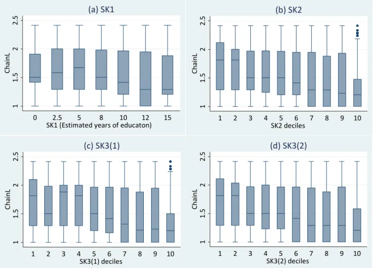
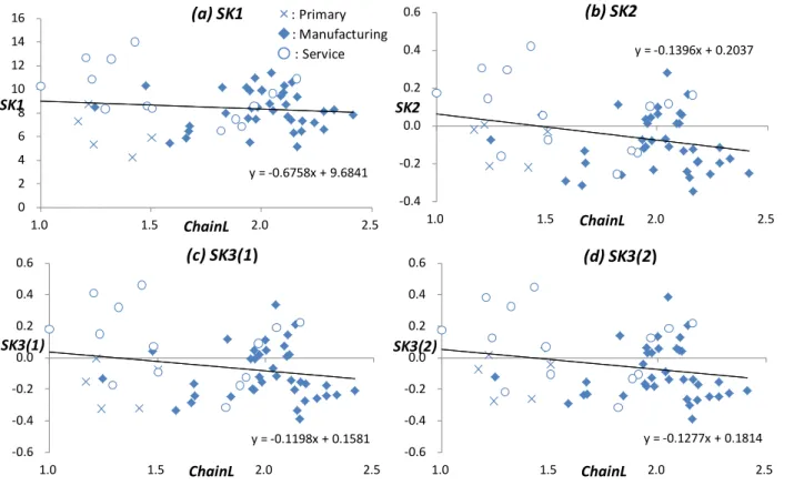
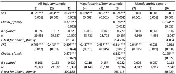
6.1 Skill-Sorting RegressionFigure 2 (individual level) and Figure 3 (industry level) present the raw
correlations between workers’ skills expressed by the four skill indices and the
industry’s production chain lengths in 1999. These two figures generally show that
high-skilled individuals work in industries with shorter production chains; that is,
negative sorting seems to occur in India. It is also evident from Figure 3 that production
chains tend to be shorter in service and primary industries than in manufacturing
industries.21
The question of whether this simple correlation remains robust even when
controlling for other factors is examined by estimating equations (4.1)–(4.3). First,
Table 1 reports the estimation results for equation (4.1), that is, the individual-level skill
sorting equation in 1999. Consistent with this paper’s negative-sorting hypothesis, the
coefficient on skill index is significantly negative in almost all specifications regardless
of skill indices, industry coverage, and control variables. I examine the manufacturing
and service industry samples, which exclude primary industries such as agriculture and
mining, because final product quality in primary industries is substantially affected by
land, weather, and natural resources, which IO tables do not include as inputs. I also
examine skill sorting within the manufacturing sector to exclude the possibility that
differences in ChainL do not represent variations in production chain length but rather
only capture differences between service and manufacturing sectors. However, it should
be noted that the sample size becomes much smaller when restricting the sample to
21
Exact ChainL figures (and Skill, ChainQ_Import, and ChainQ_Skill) for each industry are provided in Appendix Table B.1.
manufacturing. A smaller sample size results in larger standard errors in the estimated
coefficients.
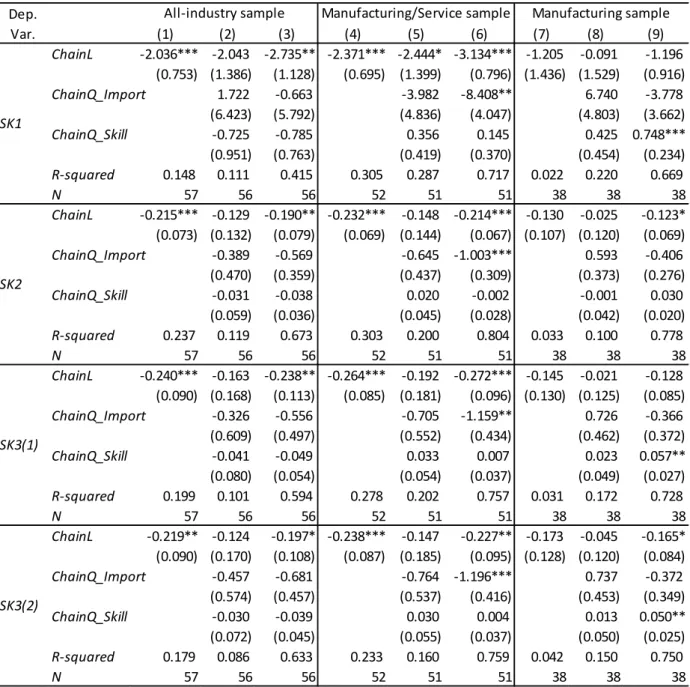
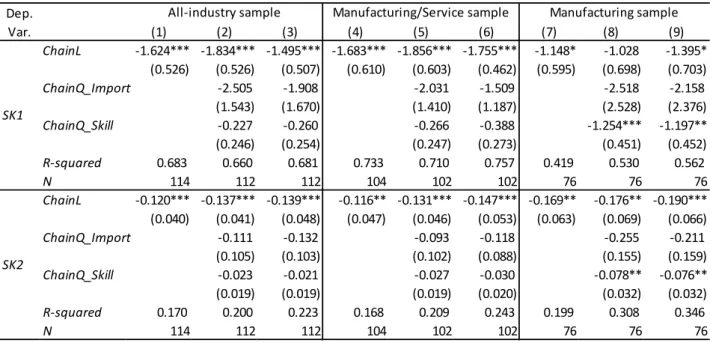
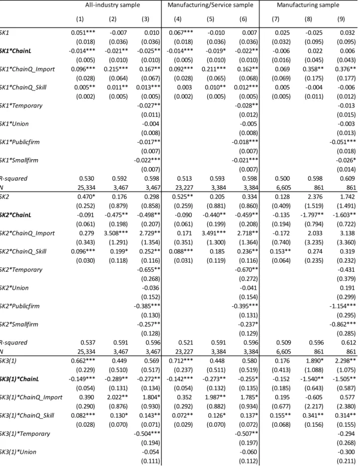
Table 2 and Table 3 report the estimation results for the industry-level skill
sorting equation for 1999 (equation (4.2)) and for the 1999–2009 panel (equation (4.3)),
respectively. In 1999, except the manufacturing-industry sample, negative sorting can
generally be observed regardless of skill indices. The negative-sorting trend is much
less clear in the manufacturing sample (Table 2). However, when controlling for
time-invariant industry characteristics using 1999–2009 panel data, negative sorting
becomes more evident regardless of variations in industry coverage (Table 3). Moreover,
a significant and unexpectedly negative sign of ChainQ_Import in column (6) of Table 2
now becomes insignificant.
ChainQ_Skill is insignificant or positively associated with an industry’s worker skill level (Skill) in the 1999 manufacturing sample. However, contrary to expectation,
the sign on the coefficient of ChainQ_Skill in the manufacturing sample turns out to be
negative in the panel regression (Table 3). This is because between 1999 and 2009,
industries with higher growth in ChainQ_Skill experienced lower growth in Skill. One
possible reason for this negative coefficient of ChainQ_Skill is that ChainQ_Skill of
industry j does not capture the quality (embodied skill level) of inputs sourced from
within its own industry (i.e., industry j). From the perspective of each worker in
industry j, the quality of inputs sourced from within industry j also matters because it
affects his or her wages. Thus, I construct
∑
∑
= k kjt kjt k kjtjt Eduy leont leont
Skilltotal
ChainQ_ ( * )/ , where subscript k includes j.
When controlling for this ChainQ_Skilltotal instead of ChainQ_Skill, the coefficients on
ChainQ_Skilltotal become positive in the panel for skill-sorting regression (Appendix Table B. 2). However, because the share of inputs sourced from within its own industry
out of the total inputs is large in general, 22 it is natural to expect that
jt
l Skillltota
ChainQ _ is positively associated with Skilljt, which is the average skill
level of workers in that same industry. Constructing a more sophisticated index to
measure the input quality that is not captured by ChainL is left for future research.
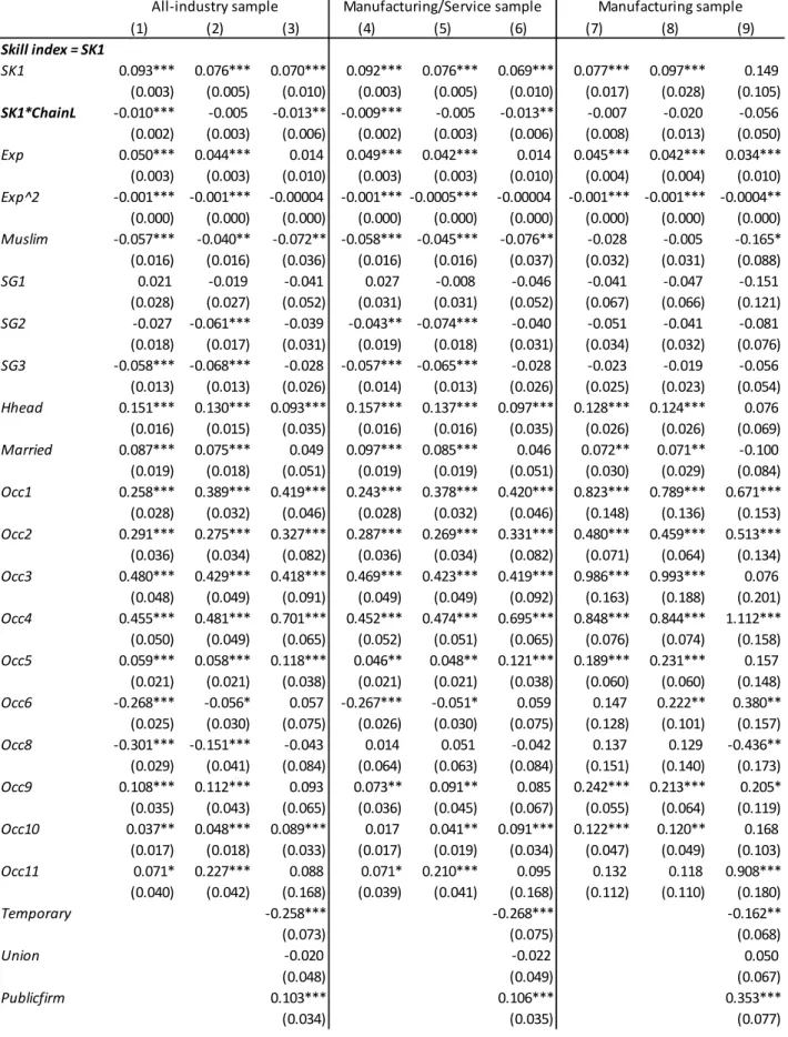
6.2 Skill Wage Premium Regression
Table 4 reports the estimation results for the skill wage premium regression
(equation (4.4)), which includes only one interaction term with Skill, that is, Skill*ChainL. A negative coefficient on this Skill*ChainL is consistent with my hypothesis that negative sorting occurs in India because the returns to skill are higher in
industries with shorter production chains.
The first column of every sample includes various individual characteristics
based on weekly status. The second column controls for industry wage premium by
adding industry dummies. The third column also controls for various job characteristics
based on yearly status.
The coefficients on Skill*ChainL are negative in some specifications but are
not so robust. The signs on coefficients for other control variables are almost consistent
with the literature and general expectations. Variables positively associated with wages
in general are skill index, experience, being household head, being married, having an
occupation other than farmer, working at a public enterprise, and being covered under
the Provident Fund (India’s social security fund). In contrast, experience squared, being
a Muslim, belonging to a disadvantaged social group, being a farmer, working in a
temporary job, working in a small firm, and living in a rural area tend to be negatively
associated with wages.
22
For instance, the length of production chains taken up by the same industry (leontjjt) accounts for 55% of the total production chain length (ChainLTjt) on average across 57 industries in 1999.
Next, other factors that may explain inter-industry skill wage differentials are
also controlled for by adding interaction terms between these factors and Skill. Table 5
reports the estimation results for all the interaction terms with Skill. Importantly, the
coefficients on Skill*ChainL become negative in most specifications; that is, returns to
skill are higher in industries with shorter production chains. Consistent with the study’s
hypothesis, returns to skill tend to increase when supplemental production chain quality
indicators (ChainQ_Import: dependence on imported inputs; ChainQ_Skil: average skill
level embodied in the inputs from other industries) are higher. This implies that input
quality affects inter-industry skill wage differentials. As expected, the skill wage
premium tends to be smaller in the public sector and in the informal sector, which is
characterized by temporary employment and small-sized firms.
7. Robustness Checks
This section provides various robustness checks, particularly for skill wage
premium regression, by (1) correcting for possible selection bias, (2) controlling for
alternative reasons for inter-industry skill wage differentials, and (3) examining a
different period (year 2009).
7.1 Selection problems
Three types of selection problems are involved in the previous skill wage
premium estimation, which was based on the sample of RWS employees. The first is the
selection into either working or non-working. The second is the selection into working
as an RWS employee or a self-employed/casual worker. The third is the selection into
each industry. The first and second selection problems are less critical because this
paper’s focus is inter-industry variations in workers’ skill levels and the skill wage
interest is considered to be RWS employees. Using an RWS-employee sample is most
appropriate to examine the skill-sorting pattern of highly skilled workers in particular
(as illustrated by the job selection example offered in the Introduction about the
most-promising IIT graduates) because most high-skilled individuals choose to work as
RWS employees. In the 1999–2000 NSS, the ratios of RWS employees, self-employed,
and casual workers among working individuals who had completed college/university
education or more are 59.1%, 38.1%, and 1.8%, respectively. Being self-employed is
also popular. However, the NSS does not provide wage data for self-employed persons.
It is also much harder to control for the diversified job characteristics of self-employed
workers.
Self-selection into industry is more critical. Individuals’ wages are not
observed for all industries; they are only observed for the single industry an individual
chooses. In other words, the group of observed individuals working in a certain industry
is not a random sample of the population. This can lead to a biased estimate for β4t in equation (4.4), which is the inter-industry skill wage differentials caused by varied
production chain lengths. Because β4t is the focus, this possible selection bias needs to be tackled.
To correct for the selection bias, I utilize the control function approach of
Wooldridge (2015: pp. 430-432), who extended the method of Garen (1984).23 As
mentioned above, the choice of ChainLij is not randomly assigned to the population.
Thus, the observed coefficient of Skill *ij ChainLij can be expressed as
individual-specific inter-industry (or more precisely, inter- ChainLij ) skill wage
differentials, gi =β4 +vi, where β is the population-average inter-4 ChainLij skill wage differentials needed to be identified and E(vi)=0. Then, the most basic version
23
I thank Jeffrey M. Wooldridge for providing me with the Stata code for the Table 1 in Wooldridge (2015).
of equation (4.4) can be re-written as24 ij ij ij ij ij ij i
ij g Skill ChainL Skill ChainL X
Wage 4 * 4 4 4 4
ln =a + +η +j +l +ε , (7.1)
where Xij is the same vector as in equation (4.1), which includes the estimated years
of work experience and its square as well as dummies for being Muslim, social groups,
household head, marriage status, residence in rural area, and Indian states of
residence.25
By substituting gi =β4 +vi into equation (7.1), the following is obtained ij ij
ij ij
ij
ij Skill ChainL Skill ChainL X
Wage 4 4 * 4 4 4 ln =a +β +η +j +l ij ij ij i Skill ChainL v * * +ε4 + . (7.2)
I assume that only lnWageijandChainLijare endogenous and that ChainLijcan be expressed by equation (4.1):
ij ij ij
ij
ij Skill X ChainL sfamily
ChainL =a1+β1 +γ1 +δ1 _ +ε1 , (4.1)
where E(ε1ij |1,Skillij,Xij,ChainL_sfamilyij)=0 . ChainL _sfamilyij (average ij
ChainL of other family members of the same gender) should be strongly correlated
with ChainLij and uncorrelated with ε . I assume that 4ij v and i ε are linearly 4ij
related to ε , that is, 1ij E(vi |ε1ij)=π1ε1ijand E(ε4ij |ε1ij)=π2ε1ij. I also assume that
i
v and ε are independent of (4ij 1,Skillij,Xij,ChainL_sfamilyij). Then, the equation to estimate the skill wage premium becomes
) , _ , , , 1 |
(lnWageij Skillij Xij ChainL sfamilyij ChainLij
E
ij ij
ij ij
ij ChainL Skill ChainL X
Skill 4 4 4 4 4 β * η j l a + + + + = ij ij ij ij Skill ChainL 2 1 1 1ε * * π ε π + + . (7.3)
Thus, β can be identified by regressing 4 lnWageijon 1, Skill *ij ChainLij, Skillij, ij
ChainL , Xij, ε1ij*Skill *ij ChainLij, and ε1ij, where ε1ij is the residual from the
regression of equation (4.1).
24
Subscript t is omitted. In order to take the control function approach, ChainLijis controlled for instead of industry dummies.
25
Experience and its square are only included when SK1 is used as a skill index.
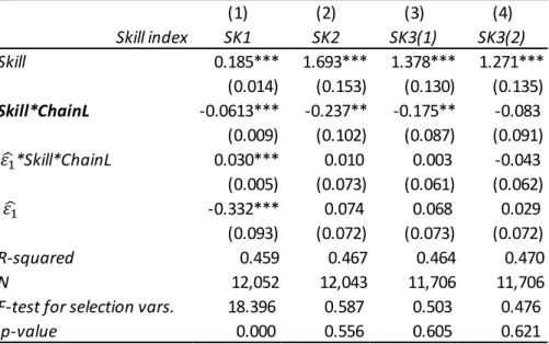
The estimation result of equation (4.1) is presented in the third column of every
sample in Table 1. The results of the F-test on the null hypothesis δ1 =0 shows that
ij
sfamily
ChainL _ is strongly associated with ChainLij . Estimation results for
equation (7.3) are reported in Table 6. First, the results of the F-test for the joint
significance of (ε1ij*Skill *ij ChainLij, ε1ij) show that selection bias exists only when using SK1 as a skill index. In cases with other skill indices, it is not necessary to correct
for selection bias. Second, even in case of SK1, the selection-corrected coefficient of
ij
ij ChainL
Skill * is still significantly negative. Thus, the results obtained in Section 6
are robust even when self-selection into industry is considered.
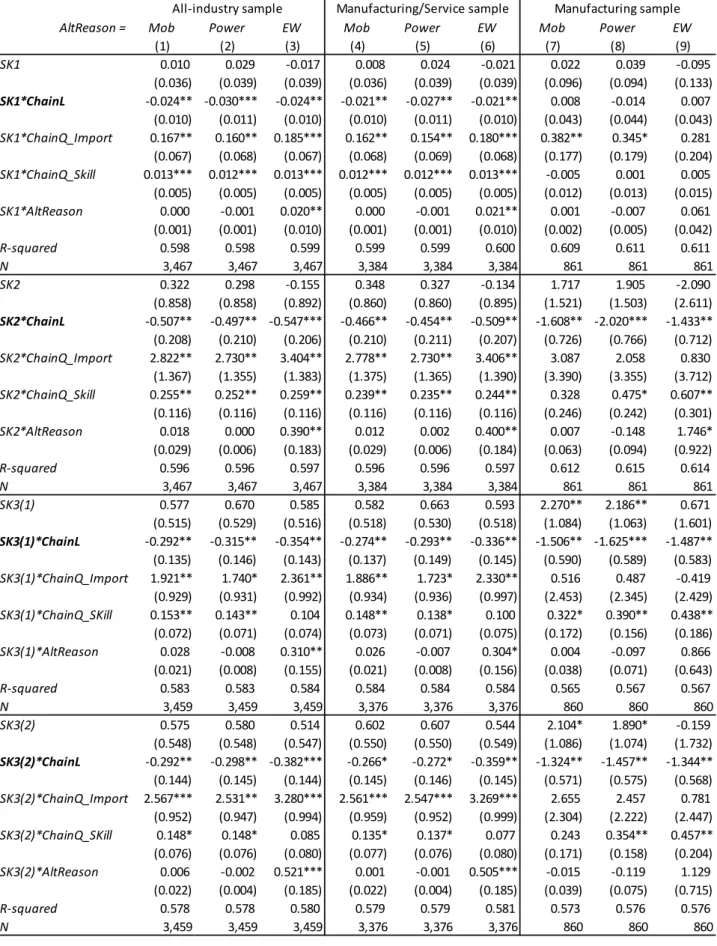
7.2 Alternative Reasons for Inter-industry Skill Wage Differentials
As mentioned in Section 2, returns to skill can vary across industries not only
because different production chain lengths among industries but also because (1) labor
mobility, (2) ability to bargain over wages, and (3) monitoring costs and necessity to
pay efficiency wages vary between high-skilled and low-skilled workers across
industries (Pavcnik et al., 2004).
Differences in labor mobility between skill groups (Mob): In a standard competitive labor-market model with perfect mobility, returns to skill are equalized
over different industries. As the labor mobility of a certain skill group becomes
lower in certain industries, the wages paid to that group in these industries deviate
from market wages. Consequently, returns to skill vary across industries. Thus, the
difference in labor mobility between high-skilled and low-skilled workers in each
industry (Mobjt) should be controlled for. As a measure forMobjt, I use the
labor-mobility gap between high-skilled and low-skilled individuals in the
sample. 26 Labor mobility, which is computed based on NSS data, is measured by
26
High-skilled workers are defined as those with lower secondary or above education (10 or more years of education completed) and low-skilled workers are those with less than a