Initial waveform optimization based on the adjoint variable and the finite element methoeds

Initial waveform optimization based on the

adjoint variable and the finite element methoeds

Takahiko Kurahashi and Shigetoshi Tai

Abstract In this study, we present the initial waveform optimization analysis based on the adjoint variable and the finite element methods. As the governing equation, a shallow-water equation is employed to simulate flow behavior, and the finite ele- ment method using the stabilized bubble function element and the Crank-Nicolson method were used for spatial and temporal discretization. In addition, the rotating cone problem is carried out to investigate the numerical of the accuracy of the bub- ble function FEM using the stabilization parameter in the SUPG method. The results of the investigation for the adjoint boundary condition are shown in this paper.

1.1 Introduction

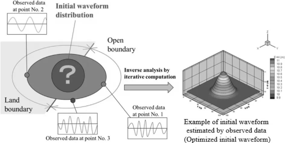
In this study, the initial waveform optimization analysis is carried out based on the adjoint variable and the finite element method. The image diagram of the waveform optimization is shown in Figure 1.1. To obtain the optimized initial waveform using the time history of observed water elevation, the performance function, i.e., the cost functional, should be defined[1],[2]. The performance function is defined as the sum of the squares of the residual between the computed and observed water elevations.

The performance function, is expressed as J = 1

2

∫ _t

t

{ η − η obs. } ^T [Q] { η − η obs. } dt, (1.1)

Takahiko Kurahashi

Nagaoka University of Technology, 1603-1 Kamitomioka, Nagaoka, Niigata 940-2188, JAPAN e- mail: [email protected]

Shigetoshi Tai

Nagaoka University of Technology, 1603-1 Kamitomioka, Nagaoka, Niigata 940-2188, JAPAN e-mail: [email protected]

1

where [Q] is the weighting diagonal matrix, η is the computed water elevation and η obs. is the observed water elevation.

The purpose of this study is to find the distribution of the initial water elevation η ^(t

) to minimize the performance function under the constraints of the shallow- water equation, the initial and the boundary conditions. Minimizing the performance function means that the computed water elevation should be as close as possible to the observed water elevation at the observation points. The results of the investiga- tion of the adjoint boundary condition in the inverse analysis based on the adjoint variable method are shown in this study. In addition, the performance function ex- tended by the governing equation, i.e., a shallow-water equation, and the adjoint variable is expressed by J

in this paper. J

is referred to as the Lagrange function and the extended performance function.

Fig. 1.1 The image diagram of the waveform optimization

1.2 Formulation by adjoint variable method

The finite element equation for the shallow-water equation is written as follows.

[M] { u ˙ _i } + [S

j (u ^adv _j )] { u _i } +g[S

] { η }

+ ν ^([H

j j ( ν

^)] { u _i } + [H

_ji ( ν

^)] { u _j } ) + f [M] { u _i } = { T _i }

in Ω ^t ∈ [t

, t _f ] (1.2)

[M] { η ˙ } + [S

(u ^adv _i )] { h } + [S

(u ^adv _i )] { η }

+[S

(h + η ^)] { u i } + [A( ν

^)] { η } = { 0 }

in Ω ^t ∈ [t

, t _f ] (1.3)

The boundary and the initial conditions are defined as follows.

u _i = u ˆ _i = ( u,0), ˆ η ⁼ η ^{ˆ on} Γ U t ∈ [t

,t _f ] (1.4) t _i = ν ^(u i, j + u j,i )n _j = (0, 0), on Γ D t ∈ [t

, t _f ] (1.5) t x = 0, ν ⁼ 0 on Γ S t ∈ [t

, t f ] (1.6) u _i (t

) = 0, η ^(t

) = η

ⁱⁿ Ω ^(1.7) Here, the parformance function, Equation (1.1), is extended by Equations (1.2), (1.3) and the adjoint variables { u

_i } and { η

} .

J

= J +

∫ _t

t

{ u

_i } ^T ([M] { u ˙ _i } + { C _i } )dt +

∫ _t

t

{ η

} ^T ([M] { η ˙ } + { D } )dt (1.8) where, { C _i } and { D } are expressed as follows.

{ C _i } = [S

_j (u ^adv _j )] { u _i } +g[S

] { η } + ν ^([H

( ν

^)] { u _i } +[H

_ji ( ν

^)] { u _j } ) + f [M] { u _i } − { T _i } t ∈ [t

,t _f ]

(1.9) { D } = [S

(u ^adv _i )] { h } + [S

(u ^adv _i )] { η }

+[S

(h + η ^)] { u _i } + [A( ν

^)] { η }

t ∈ [t

,t _f ] (1.10)

To obtain the stationary condition of J

, the first variation of the extended perfor- mance function, Equation (1.11), is calculated. By calculating the first variation of the derivation of stationary condition extended performance functionm the follow- ing equation can be obtaind.

δ ^J

^{= 0 (1.11)}

The Adjoint equations are written as follows.

− [M ] ^T { u ˙

_i } + [ ∂ ^C i

∂ ^u i

] T

{ u

_i } + [ ∂ ^D

∂ ^u i

] T

{ η

} = { 0 }

in Ω ^t ∈ [t

, t _f ] (1.12)

− [M] ^T { η ˙

} + [ ∂ ^C i

∂η ] T

{ u

_i } +

[ ∂ ^D

∂η ] T

{ η

} + { η − η obs. } ^T [Q] = { 0 }

in Ω ^t ∈ [t

, t _f ] (1.13)

Here, the boundary and terminal conditions are denoted as follows.

u

= 0 t _y

= 0 on Γ U t ∈ [t

,t _f ] (1.14) t _i

= (0, 0) on Γ D t ∈ [t

,t _f ] (1.15) ν

^{= 0 t} x

= 0 on Γ S t ∈ [t

, t _f ] (1.16) u

_i (t _f ) = 0 η

^(t f ) = 0 in Ω ^(1.17) In addition, the gradient vector of the extended performance function with respect to the initial water elevation can be written as following equation.

{ ∂ ^J

∂η ^(t

) }

= [M] ^t { η

^(t

) } in Ω ^(1.18) Therefore, the initial water elevation can be updated by using Equation (1.18).

The update equation of the initial waveform can be written as follows.

{ η ^(t

) }

= { η ^(t

) }

+ α

{ ∂ ^J

∂η ^(t

) }

in Ω ^(1.19)

1.3 Rotating cone problem

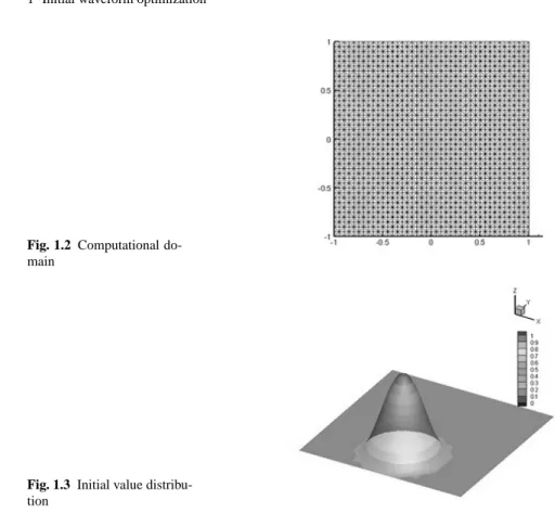
In this section, the rotating cone problem is carried out to investigate the advantages of the bubble function FEM using stabilization parameter in SUPG method. As the governing equation, the advection equation is employed. The spatial distribution of variable φ represented in the equation (1.20) (see Figure 1.3) is given as shown in Figure 1.2. The advection velocity field given by the u = − y and v = x. The bubble function element without the stabilization parameter is employed in case 1, the bubble function element with the stabilization parameter which is equivalent to that by the SUPG method is employed in case 2.

φ ⁼

{ 0.5(cos(2 π ^{r) + 1) r} ≤ 0.5

0 r > 0.5 (1.20)

Fig. 1.2 Computational do- main

Fig. 1.3 Initial value distribu- tion

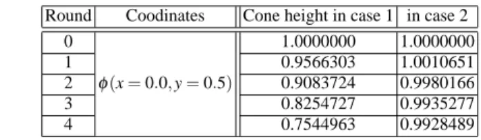
Computational conditions are shown in Table 1.1. In addition, computational re- sults are shown in Table 1.2. It is found that the numerical damping can be controlled by using the bubble function element with the stabilization parameter.

Table 1.1 Computational conditions

Number of nodes 1,681

Number of elements 3,200

Time increments 0.001

Time step 25,120

Table 1.2 Comparison of cone height in case 1 and 2

Round Coodinates Cone height in case 1 in case 2

0 1.0000000 1.0000000

1 0.9566303 1.0010651

2 φ (x = 0.0,y = 0.5) 0.9083724 0.9980166

3 0.8254727 0.9935277

4 0.7544963 0.9928489

1.4 Numerical experiment

1.4.1 Computational flow of waveform optimization

The computational flow of waveform optimization is shown below.

1. Assume initial water elevation η ^(t

)

. 2. Compute state equation.

3. Compute performance function J

. 4. Compute adjoint equation.

5. Update initial water elevation η ^(t

)

by gradient vector g

.([W

] ^T { η ^(t

)

} = [W

] ^T { η ^(t

)

} + { g

} )

6. Check of convetgence; if | J

− J

| < eps, then stop, else go to step 7.

7. Compute state equation.

8. Compute performance function J

. 9. Update weighting parameter W

.

a. if J

< J

, then W

= W

× 0.9 and go to step 4.

b. if J

> J

, then W

= W

× 2.0 and go to step 5.

1.4.2 Results of numerical experiments

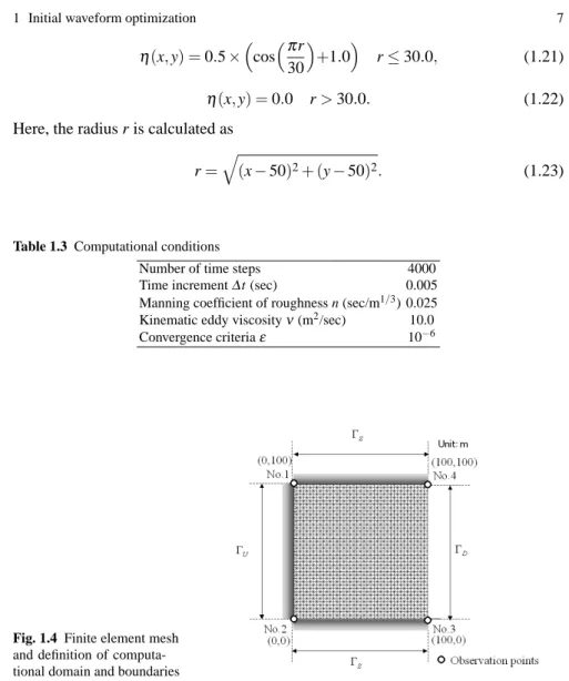
The purpose of this study is to determine the distribution of water elevation to bring the computed water elevation close to the observed water elevation at the observa- tion points based on the adjoint variable method. The finite element mesh and the location of observation points are shown in Fegure 1.4. The total number of nodes and elements are respectively 1681 and 3200. The computational conditions for this analysis are listed in Table 1.3. The weighting constant Q at the observation point is 1.0 and at the other points are 0.0. In this study, the artificial observed water el- evation obtained by using the exact initial water elevation shown in Figure 1.5 is employed. The mean water depth h is set at 10.0 m in the computational domain.

The distribution of the initial water elevation shown in Figure 1.5, is expressed in

the form of the following equations.

η ^{(x, y) = 0.5} × ( cos

( π ^r 30 )

+1.0 )

r ≤ 30.0, (1.21)

η ^{(x, y) = 0.0 r > 30.0. (1.22)}

Here, the radius r is calculated as r =

√

(x − 50)

+ (y − 50)

. (1.23)

Table 1.3 Computational conditions

Number of time steps 4000

Time increment ∆ t (sec) 0.005

Manning coefficient of roughness n (sec/m

) 0.025 Kinematic eddy viscosity ν (m

/sec) 10.0

Convergence criteria ε 10

Fig. 1.4 Finite element mesh and definition of computa- tional domain and boundaries

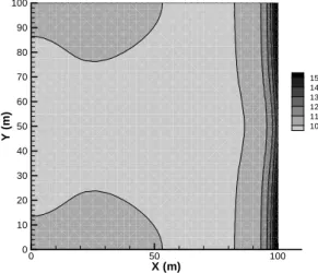
If the adjoint boundary condition on the open boundary Γ D is defined as the ad- joint flux s _x = 0.0 the distribution of the gradient

^J

0)

at the first iteration is ob- tained, as shown in Figure 1.6. The adjoint flux s _x is related variable with respect to the flow quantity flux for x direction. In this case, the iterative computation for the inverse analysis is not carried out, since the gradient distribution is not appro- priately expressed. The distribution of the initial water elevation is obtained as the linear combination for the gradient vector with respect to the initial water elevation.

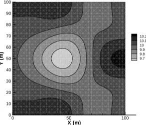
Therefore, if the gradient vector at the first iteration is not obtained precisely, the inverse analysis computation cannot be continued. In this case, it appears that if the gradient value is concentrically distributed, the analysis can be carried out. Here, let us consider the case where the adjoint boundary condition on the open boundary Γ D

is defined as λ x = 0.0. The adjoint variable λ x is related variable with respect to the

Fig. 1.5 Distribution of initial water depth ( η + h) (Exact solution for estimation of initial water elevation)

10 10.5 11

E+H(m)

0 20 40 60 80 100

X (m) 0

20 40

60 80

100 Y (m)

X Y

Z

E+H (m) 11 10.9 10.8 10.7 10.6 10.5 10.4 10.3 10.2 10.1 10 9.9

flow velocity for x direction. Consequently, the gradient distribution is obtained as shown in Figure 1.7. In this case, the iterative computation for the inverse analysis is carried out, and the distribution of the initial water elevation is appropriately ob- tained.

X (m)

Y(m)

0 50 100

0 10 20 30 40 50 60 70 80 90 100

15 14 13 12 11 10

Fig. 1.6 Distribution of gradient of extended performance function with respect to initial water

elevation ( conventional method )

X (m)

Y(m)

0 50 100

0 10 20 30 40 50 60 70 80 90 100

10.2 10.1 10 9.9 9.8 9.7

Fig. 1.7 Distribution of gradient of extended performance function with respect to initial water elevation ( present method )

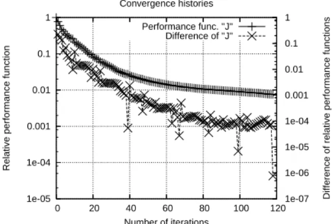
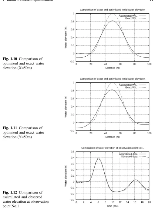
The computational results are shown as follows. Figure 1.8 shows the variation in the performance function. It can be seen that the performance function decreases and converges. This means the computed water elevation is close to the observed water elevation. The distribution of the initial water elevation, shown in Figure 1.9, can thus be obtained. Figures 1.10 and 1.11 show a comparison of the initial water level between the computed and the exact values on the lines X = 50.0 m and Y = 50.0 m. It can be seen that the computed initial water elevation is lower than the exact initial water elevation.

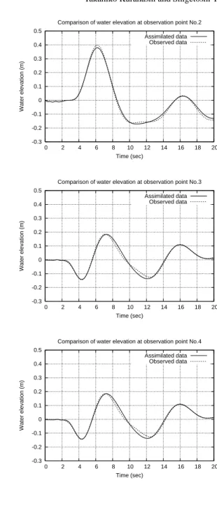
Figures 1.12 - 1.15 show the time histories of water elevation at the observation points Nos. 1 - 4. The solid line indicates the assimilated water elevation and the broken line indicates the observed water elevation. At all the observation points, the assimilated water elevation is in good agreement with the observed water elevation.

It is seen in Figures 1.12 and 1.13 that there is difference early on. It appears that

this is not a type of the error in the computation of the shallow water flow. This

is because the observed data in Figures 1.12 and 1.13 are also obtained by using

the shallow water code in the same way as the code used in the computation of

the estimation for the initial water elevation. There is thus the possibility of a kind

of numerical error in the computation of the inverse analysis, since the assimilated

data at No. 3 was the same as the data at No. 4. In this computation, the adjoint

boundary condition on the open boundary Γ D is defined as λ x = 0.0. The adjoint

flux s _x integrated in time duration [t

,t _f ] and on the open boundary Γ D must there-

fore be zero to satisfy the stationary condition δ ^J

⁼ 0, under conditions where the

performance function converges. This is because, in the equation of the first varia-

tion of the extended performance function, the term for the adjoint flux integrated

1e-05 1e-04 0.001 0.01 0.1 1

0 20 40 60 80 100 120 1e-07

1e-06 1e-05 1e-04 0.001 0.01 0.1 1

Relative performance function Difference of relative performance functions

Number of iterations Convergence histories

Performance func. "J"

Difference of "J"

Fig. 1.8 Variation of performance function and absolute value of difference of performance func- tion between (l) and (l + 1) iterations

10 10.5 11

E+H(m)

0 20 40 60 80 100

X (m) 0

20 40

60 80

100 Y (m)

X Y

Z

E+H (m) 11 10.9 10.8 10.7 10.6 10.5 10.4 10.3 10.2 10.1 10 9.9

Fig. 1.9 Distribution of optimized initial water depth ( η + h)

in time and on the open boundary should be zero. In general, the adjoint flux on

the open boundary is defined as zero to satisfy the stationary condition. However, in

this study, the initial water elevation can be obtained by computation in which the

adjoint boundary condition on the open boundary is defined as λ x = 0.0. Therefore,

it is necessary to investigate whether the value of the adjoint flux integrated in time

and on the open boundary is headed for zero if the type of adjoint boundary condi-

tion is changed, i.e., the adjoint boundary condition on the open boundary is defined

Fig. 1.10 Comparison of optimized and exact water elevation (X=50m)

-0.2 0 0.2 0.4 0.6 0.8 1

0 20 40 60 80 100

Water elevation (m)

Distance (m)

Comparison of exact and assimilated initial water elevation Assimilated W.L.

Exact W.L.

Fig. 1.11 Comparison of optimized and exact water elevation (Y=50m)

-0.2 0 0.2 0.4 0.6 0.8 1

0 20 40 60 80 100

Water elevation (m)

Distance (m)

Comparison of exact and assimilated initial water elevation Assimilated W.L.

Exact W.L.

Fig. 1.12 Comparison of assimilated and observed water elevation at observation point No.1

-0.3 -0.2 -0.1 0 0.1 0.2 0.3 0.4 0.5

0 2 4 6 8 10 12 14 16 18 20

Water elevation (m)

Time (sec)

Comparison of water elevation at observation point No.1 Assimilated data

Observed data

Fig. 1.13 Comparison of assimilated and observed water elevation at observation point No.2

-0.3 -0.2 -0.1 0 0.1 0.2 0.3 0.4 0.5

0 2 4 6 8 10 12 14 16 18 20

Water elevation (m)

Time (sec)

Comparison of water elevation at observation point No.2 Assimilated data

Observed data

Fig. 1.14 Comparison of assimilated and observed water elevation at observation point No.3

-0.3 -0.2 -0.1 0 0.1 0.2 0.3 0.4 0.5

0 2 4 6 8 10 12 14 16 18 20

Water elevation (m)

Time (sec)

Comparison of water elevation at observation point No.3 Assimilated data

Observed data

Fig. 1.15 Comparison of assimilated and observed water elevation at observation point No.4

-0.3 -0.2 -0.1 0 0.1 0.2 0.3 0.4 0.5

0 2 4 6 8 10 12 14 16 18 20

Water elevation (m)

Time (sec)

Comparison of water elevation at observation point No.4 Assimilated data

Observed data

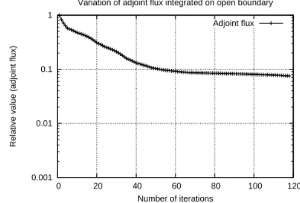
as λ x = 0.0. Figure 1.16 shows the history of the adjoint flux ^∫ _t ^t

^∫

D

s _x d Γ ^{dt. The} value of the adjoint flux is reduced by 92.5% and can be close to zero. The adjoint flux on the open boundary has to theoretically converge to zero to satisfy the station- ary condition. However, the adjoint flux on the open boundary does not completely converge to zero, since this computation is carried out numerically and iteratively.

In this computation, the adjoint flux on the open boundary can consequently be re- duced sufficiently compared with the value at the first iteration, and can approach zero, as shown in Figure 1.16. It therefore appears that if the data assimilation prob- lem with open boundary can’t be solved based on the traditional method, the present method can be useful in solving for the problem.

Fig. 1.16 History of adjoint flux s

integrated in time and on open boundary Γ

0.001 0.01 0.1 1

0 20 40 60 80 100 120

Relative value (adjoint flux)

Number of iterations

Variation of adjoint flux integrated on open boundary Adjoint flux

1.5 Conclusions

In this study, the initial waveform optimization analysis was carried out based on the adjoint variable and the finite element method. A shallow-water equation was employed to simulate flow behavior, and the finite element method using the stabi- lized bubble function element and the Crank-Nicolson method were used for spatial and temporal discretization. The initial water elevation optimization problem was solved as a minimization problem of the performance function, expressed as the sum of the squares of the residual between the computed and the observed water el- evations. The Sakawa-Shindo method was employed as the minimization technique of the performance function.

In the numerical experiment, an investigation into the definition of the boundary

condition with respect to the adjoint variables on the open boundary was carried

out to optimize the initial waveform. Consequently, the optimized initial waveform

could be obtained.

References

1. T.Kurahashi and M.Kawahara, Examinations for terminal condition of Lagrange multiplier for heat transfer control problems, Int. J. Numer. Meth. Eng., 73 (2008), 982-1009.

2. R.Glowinski and Q.He, A Least-Squares/Fictitious Domain Method for Linear Elliptic Problems with Robin Boundary Conditions, Commun. Comput. Phys., 9 (2011), 587-606.

3. T.Kempe and J.Frohlich, An improved immersed boundary method with direct forcing for the simulation of particle laden flows, J. Comput. Phys., 231 (2012), 3663-3684.

4. Y.Sakawa and Y.Shindo, On global convergence of an algorithm for optimal

control, IEEE Transactions on Automatic Control, 25 (1980), 1149-1153.