Shape optimization analysis in viscous flow fields considering rotational body based on the adjoint variable and the finite element methods

(1)

The World Congress of Structural and Multidisciplinary Optimization, May 20-24, 2019, Beijing, China

Shape optimization analysis in viscous flow fields considering rotational body based on the adjoint variable and the finite element methods

Yuta Ozeki¹*, Takahiko Kurahashi¹ and Eiji Katamine²

1Dept. of Mechanical Engineering, Nagaoka University of Technology, Niigata, Japan

* Corresponding author: [email protected]

2 Dept. of Mechanical Engineering, National Institute of Gifu College, Gifu, Japan

Abstract

In this study, we present shape optimization analysis considering rotational body in flow field based on the adjoint variable and the finite element methods. The purpose of this study is to obtain optimal shape so as to close to the target velocity at target regions. The Freefem++ is used in calculation of the optimal shape, and some numerical results are shown in this study.

Keywords: Shape optimization, Adjoint variable method, Finite element method, Rotational body.

1. Introduction

In this study, numerical experiments for shape optimization problem including rotational body is performed. The shape optimization problem in Stokes flow is theoretically explained, and it is known that the optimal shape is a rugby ball shape in case of the drag minimization problem in Stokes flow [1]. In addition, it is known that the distribution of the gradient of the Lagrange function with respect to coordinate is oscillated on the design boundary, and the traction method was developed to control the numerical oscillation [2]. The traction method is applied to shape optimization problem considering minimization of dissipation energy [3] and so on, and it is confirmed that smoothed gradient distribution can be appropriately calculated, and the optimal shape can be numerically obtained. The shape optimization analysis of body located in unsteady-state viscous flow field is also investigated by Yagi and Kawahara [4], and the other smoothing technique is employed in this study [5]. Based on these research results, we investigate the shape optimization problem considering rotational body using Freefem++ [6].

2. Formulation for shape optimization based on the adjoint variable method

In this study, the performance function is defined as shown in Eq. (1) considering the objective that the flow velocity is close to the target velocity at target regions.

𝐽 = 12 ∫ ∫ 𝑄_𝑖(𝑢𝑖− 𝑢_{𝑖(𝑡𝑎𝑟𝑔𝑒𝑡)})²𝑑𝛺𝑑𝑡

𝛺 𝑡_𝑓

𝑡₀ (1)

where Qi, ui and ui(target) denote weight constant, computed flow velocity and target flow velocity. t0, tf and Ω denote initial time, terminal time and computational domain. The incompressible Navier-Stokes equation shown in Eqs. (2) and (3), initial and boundary conditions shown in Eqs. (4), (5) and (6) are introduced as constraint conditions for the performance function. Moreover, the area constraint condition shown in Eq. (7) is considered.

𝑢̇_𝑖+ 𝑢_𝑗𝑢_𝑖,𝑗+ 𝑝_,𝑖− 1𝑅𝑒𝑢_{𝑖,𝑗𝑗}= 0 in 𝑡 ∈ [𝑡0, 𝑡_𝑓] in 𝛺 (2)

𝑢_𝑖,𝑖= 0 in t ∈ [𝑡0, 𝑡_𝑓] in 𝛺 (3)

𝑢_𝑖= 𝑢̂_𝑖 at 𝑡 = 𝑡₀ in 𝛺 (4)

𝑢_𝑖= 𝑢̂_𝑖 in 𝑡 ∈ [𝑡0, 𝑡_𝑓] on 𝛤₁, 𝛤_{𝑟𝑜𝑡𝑎𝑡𝑖𝑜𝑛} and 𝛤_{𝑑𝑒𝑠𝑖𝑔𝑛} (5) 𝑡_𝑖= 𝑡̂ = {−𝑝𝛿_𝑖 ^𝑖𝑗+ 1

𝑅𝑒𝑢_𝑖,𝑗} 𝑛^𝑗 in 𝑡 ∈ [𝑡0, 𝑡_𝑓] on 𝛤₂ (6)

(2)

∑ 𝐴^𝑖

𝑚𝑥 𝑖=1

= 𝐴_{𝑖𝑛𝑖𝑡𝑖𝑎𝑙} in 𝛺 (7)

where ui , p , Re , δij and ni indicate flow velocity, pressure, Reynolds number, Dilac’s delta function and direction cosine of the unit outward normal of the boundary, respectively. Γ1, Γ2, Γrotation and Γdesign represent the Dirichlet, the Neumann, the rotational body and the design boundaries. On the rotational boundary, the flow velocity gives as u1 = -ωrsinθ, u2 = ωrcosθ. The parameters ω, r and θ indicate the angular velocity, distance from rotational center point and angle for rotational center point, respectively. In addition, in Eq. (7), mx and Ainitial express the total number of elements and the area of whole domain excepting for rotational body at initial iteration. The boundary condition given on Γrotation is referred to as the adhesive boundary condition. Introducing the adjoint variables, the performance function is extended as Eq. (8).

Eq. (8) is referred to as the Lagrange function.

𝐽^∗= 𝐽 + ∫ ∫ 𝑢^𝑡^𝑓 _𝛺 ^𝑖^∗{𝑢̇^𝑖+ 𝑢_𝑗𝑢_𝑖,𝑗+ 𝑝_,𝑖− 1𝑅𝑒𝑢_{𝑖,𝑗𝑗}}𝑑𝛺𝑑𝑡

𝑡₀ + ∫ ∫ 𝑝^∗𝑢_𝑖,𝑖𝑑𝛺𝑑𝑡

𝛺 𝑡_𝑓

𝑡₀ (8)

where ^∗ and ^∗ indicate the adjoint variables for the flow velocity and pressure respectively. The first variation of the Lagrange function has to be zero to satisfy the stationary condition. From the first variation of the Lagrange function, the adjoint equation and the conditions for adjoint variables are obtained. The governing equation and the adjoint equations are repeatedly computed for each shape update. The shape update is carried out by using the gradient of Lagrange function with respect to coordinate on the design boundary, and the traction method is applied to control oscillation of the gradient value.

3. Numerical experiment

The shape identification analysis considering a rotational body is carried out. The computational condition is shown in Table 1, and the computational model and the boundary conditions are shown in Fig. 1. The non-dimensional angular velocity ω are given as 2π, 6π and 10π. The finite element mesh, i.e., initial mesh in shape identification analysis, is shown in Figs. 2 and 3. The target shape in the shape identification analysis is shown in Fig. 4, and the computed flow velocity in target regions are used in the shape identification analysis. In target regions, the weighting constant Qi is given as 1.0 in target regions, otherwise the weighting constant Qi is given as 0.0. In addition, finite element meshes which are used to obtain the target velocity in case of ω = 2π, 6π and 10π are shown in Figs. 5 and 6.

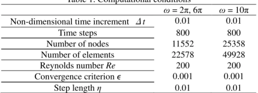
As the computational result, Fig. 7, show the variation of both performance function and area of target domain. It is seen that the value of the performance function gradually decreases and converges in all angular velocity cases, and area of target domain keeps constant. The comparison of initial shape and identified shape is shown in Fig. 8. It is seen that the initial shape is approach to the target shape in all cases, and the identified shape doesn’t depend on the non-dimensional angular velocity ω are given as 2π, 6π and 10π. Figures 9 - 11 show the time history of the velocity at center point in target regions A, B and C, respectively. In all angular velocity cases, it is found that the result in case of identified shape is approach to the result in case of target shape in comparison with the result in case of initial shape.

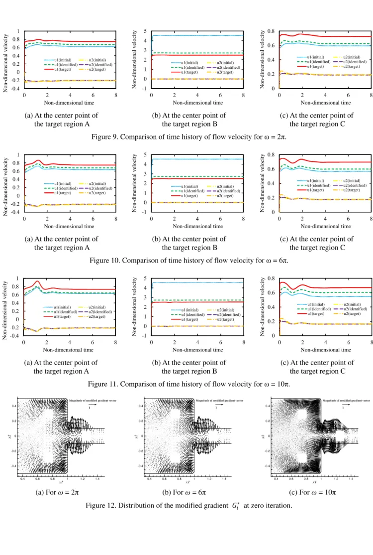
From results of numerical experiments, it can be said that the appropriate shape can be obtained such that the computed velocity is close to the target velocity. On the other hand, it is found that it is not usual that the target shape can be appropriately obtained. Looking at the results in detail, in Fig.11, it is seen that the difference between non-dimensional velocity at initial iteration and target velocity is big at target region B, while that is small at target regions A and C. In addition, it is found that the identified shape is close to target shape near target region B, and the identified shape is distant from target shape near target regions A and C. Namely, from this fact, it appears that the sensitivity for shape update become big in case that the difference between the non-dimensional velocity at initial iteration and target velocity is big.

(See Fig. 12.)

Table 1. Computational conditions

ω = 2π, 6π ω = 10π Non-dimensional time increment Δt 0.01 0.01

Time steps 800 800

Number of nodes 11552 25358

Number of elements 22578 49928

Reynolds number Re 200 200

Convergence criterion ϵ 0.001 0.001

Step length η 0.01 0.01

(3)

Figure 1. Computational model, target regions and boundary condition.

Figure 2. Finite element mesh of initial shape for ω = 2π and ω = 6π.

Figure 3. Finite element mesh of initial shape for ω = 10π.

Figure 4. Target shape

Figure 5. Finite element mesh of target shape for ω = 2π and ω = 6π

Figure 6. Finite element mesh of target shape for ω = 10π

Figure 7. Variation of both performance function

and area. Figure 8. Comparison of initial shape identified shape

and target shape.

R0.05

0.1 0.25 0.25

0.5 0.5

Γ

Γrotation 1

Γ1

Γdesign

Γ₂ Γ1

Γ1

=1-4x u1

=0 u2

2 2

x₁ x₂

region A

1.5 (-1.5,0.5)

(-1.5,-0.5)

0.25 0.1

0.25 0.4

0.2 0.1 0.4

0.1 0.1

0.25

0.4

R0.05

region C

region B ui=0

ω

0.5

0.5 1.0

x1

x2

region A

1.5 (-1.5,0.5)

(-1.5,-0.5)

0.4 0.2 0.4

region C region B

0.5

0 20 40 60 80 100 120

0 5 10 15 20 25 30 35

Area (ω= 2π) Area (ω= 6π) Area (ω= 10π)

Performance function (ω= 2π) Performance function (ω= 6π) Performance function (ω= 10π)

Number of iteration

Ratio (%)

0.4 0.6 0.8 1 1.2 1.4

-0.4 -0.2 0 0.2 0.4

Identified shape forω = 10π Initial shape

Identified shape forω = 6π Identified shape forω = 2π

Target shape

(4)

(a) At the center point of the target region A

(b) At the center point of the target region B

(c) At the center point of the target region C Figure 9. Comparison of time history of flow velocity for ω = 2π.

(a) For ω = 2π (b) For ω = 6π (c) For ω = 10π

Figure 12. Distribution of the modified gradient ^∗ at zero iteration.

-0.4 -0.2 0 0.2 0.4 0.6 0.8 1

0 2 4 6 8

u1(initial) u2(initial) u1(identified) u2(identified) u1(target) u2(target)

Non-dimensional time

Non-dimensionalvelocity

-1 0 1 2 3 4 5

0 2 4 6 8

0 0.2 0.4 0.6 0.8

0 2 4 6 8

-0.4 -0.2 0 0.2 0.4 0.6 0.8 1

0 2 4 6 8

-1 0 1 2 3 4 5

0 2 4 6 8

0 0.2 0.4 0.6 0.8

0 2 4 6 8

-0.4 -0.2 0 0.2 0.4 0.6 0.8 1

0 2 4 6 8

-1 0 1 2 3 4 5

0 2 4 6 8

0 0.2 0.4 0.6 0.8

0 2 4 6 8

0.4 0.6 0.8 1 1.2 1.4

-0.4 -0.2 0 0.2 0.4

0.4 0.6 0.8 1 1.2 1.4

-0.4 -0.2 0 0.2 0.4

0.4 0.6 0.8 1 1.2 1.4

-0.4 -0.2 0 0.2 0.4

(5)

4. Conclusion

In this paper, we presented shape optimization problems considering rotational body in flow field based on the adjoint variable and the finite element methods. The incompressible Navier-stokes equation was employed as the governing equation, and the Galerkin method and the backward difference method was applied to discretize the governing and the adjoint equations in space and time, respectively. In the numerical experiments, numerical tests for shape identification considering rotational body was carried out. Consequently, it was found that the rotational velocity doesn’t significantly affect the identified shape.

Acknowledgements

This work was supported by the Program for High Reliable Material Design and Manufacturing at Nagaoka University of Technology.

References

1. Pironneau, O., On optimum profiles in Stokes flow, Journal of Fluid Mechanics, 59, Part1, pp.117-128, 1973.

2. Azegami, H., Solution to domain optimization problems, Transactions of the Japan Society of Mechanical Engineers, Series A, 60, 574, 1479-1486, 1994 (in Japanese).

3. Katamine, E., Azegami, H., Tsubata, T. and Ito, S., Solution to shape optimization problems of viscose flow field, International Journal of Computational Fluid Dynamics, 19, 1, 45-51, 2005 (in Japanese).

4. Yagi, H. and Kawahara, M., Optimal shape determination of a body located in incompressible viscous flow, Computer Methods in Applied Mechanics and Engineering, Vol.196, (2007), pp.5084-5091.

5. Jameson, A., Aerodynamic shape optimization using the adjoint method, Lecture at the Von Karman Institute, Brussels, 2003.

6. Hecht, F., New development in FreeFem++, Journal of Numerical Mathematics, 20, 3-4, 251-265, 2012.