Shape optimization of corrosion using
temperature history observed on reinforcement concrete based on the adjoint variable and the finite element methods
Takahiko KURAHASHI, Takumi KUROSAWA, Hideki OSHITA, Kotaro MARUOKA and Tetsuro IYAMA
Abstract In this study, we present the shape estimation problem of reinforcement corrosion in concrete using the observed temperature on concrete surface based on the optimal control theory, i.e., the adjoint variable method, and the finite element method. The investigation of the dependency of the corrosion shape for the com- putational condition by changing the initial corrosion length was carried out in this study.
1.1 Introduction
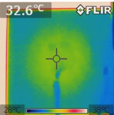
It is known that if there is defect, i.e., the cavity, the corrosion and etc., in the struc- ture and the structure is heated from the bottom surface, and the upper surface of the defect become to difference temperature comparing to the case without the defect (See Figure 1.1). However, the shape of the defect can not be directly determined by the observed temperature data on the structure. Therefore, in this study, the in- Takahiko KURAHASHI
Nagaoka University of Technology, 1603-1 Kamitomioka, Nagaoka, Niigata, Japan, e-mail: kura- [email protected]
Takumi KUROSAWA
Graduate School of Nagaoka University of Technology, 1603-1 Kamitomioka, Nagaoka, Niigata, Japan, e-mail: [email protected]
Hideki OSHITA
Chou University, 1-13-27 Kasuga, Bunkyou, Tokyo, Japan, e-mail: [email protected] Kotaro MARUOKA
Graduate School of Nagaoka University of Technology, 1603-1 Kamitomioka, Nagaoka, Niigata, Japan, e-mail: [email protected]
Tetsuro IYAMA
Nagaoka National College of Technology, 888 Nishikatakai, Nagaoka, Niigata, Japan, e-mail:
[email protected]
1
verse analysis is carried out to estimate the appropriate corrosion shape such that computed temperature is close to the observed temperature at the target point on the concrete surface in three-dimensional domain.
If the inverse problems are solved, the sensitivity equation method[1] and the adjoint variable method[2],[3],[4] , i.e., the optimal control theory, are frequently employed. In case that the number of the unknown parameters in the inverse prob- lem is few, the sensitivity equation method is suitable. On the other hand, if there are a lot of the unknown parameters the adjoint variable method is suitable for the inverse analysis. In this study, the adjoint variable method is applied to solve this problem, because it is necessary to compute a lot of unknown parameters which is equivalent to the number of the coordinates at all nodal points on the corrosion sur- face. The finite element method is applied to simulate the temperature distribution in the concrete. In this study, the numerical experiments are carried out to investi- gate the influence of the initial corrosion length in the inverse analysis for the final corrosion shape obtained by iterative computation. The image diagram of the shape determination of defect is shown in Figure 1.2.
Fig. 1.1 Heat image in case that there is defect in center of structure
Fig. 1.2 Image diagram of the shape determination of defect
1.2 Test example for non-destructive inspection based on temperature measurement
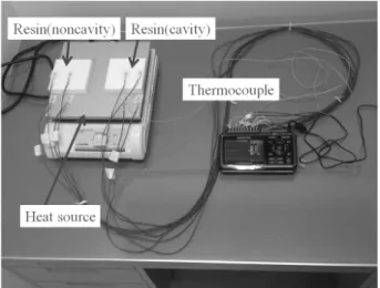
Figure 1.3 indicates the photo of experiment. There is test piece on the heater, and time history of temperature is measured on the top of the test piece. The drawing of the test piece is shown in Figure 1.4. The test piece consists of the resin, and there is a cavity at center of test piece. The size of the test piece is 100mm × 100mm × 20mm.
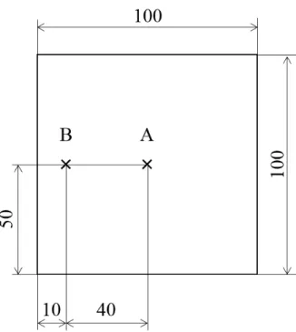
The experiment was carried out under the condition that the temperature on heater is set 50degs. The measurement points A and B are illustrated in Figure 1.5.
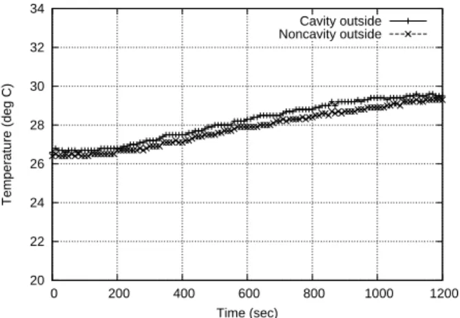
Figures 1.6 and 1.7 indicate the time history of temperature at points A and B, re- spectively. It is found that the highest temperature is obtained in case that there is a cavity in the test piece (See Figure 1.6.) From this result, it can be said that the temperature on top of the teat piece is changed if there is defect in the test piece.
Fig. 1.3 Photo of experiment
Fig. 1.4 Drawing of test piece
Fig. 1.5 Location of measurement points on upper surface
20 22 24 26 28 30 32 34
0 200 400 600 800 1000 1200
Temperature (deg C)
Time (sec)
Cavity inside Noncavity inside
Fig. 1.6 Time history of temperature on resin surface at point A
20 22 24 26 28 30 32 34
0 200 400 600 800 1000 1200
Temperature (deg C)
Time (sec)
Cavity outside Noncavity outside
Fig. 1.7 Time history of temperature on resin surface at point B
1.3 Shape determination analysis of reinforcement corrosion based on adjoint variable and finite element methods 1.3.1 Heat transfer analysis based on FEM
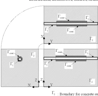
The finite element analysis is carried out to calculate the temperature distribution on the concrete surface. Figure 1.8 shows the computational model and the bound- ary definition. Γ 1 and Γ 2 denote the boundaries on which the temperature and the heat flux are respectively given, and Γ cont. indicates the surface boundary of the re- inforcement corrosion.
The heat transfer equation shown in Equation (1.1) is employed in this study.
ρ c ˙ φ − κφ ,ii = 0 (1.1)
where ρ is the density, c is the specific heat, κ is the thermal conductivity, φ is the temperature. The initial and the boundary conditions are defined as Equations (1.2) - (1.4).
φ (t 0 ) = φ ˆ 0 in Ω (1.2)
φ = φ ˆ on Γ 1 (1.3)
b = κφ ,i n i = ˆb on Γ 2 (1.4)
where n i denotes the cosine of the unit outward normal of the boundary, b denotes the heat flux.
The finite element formulation using the tetrahedron element is applied to com-
pute the heat transfer equation. The finite element equation is consequently derived
as shown in Equation (1.5).
Fig. 1.8 Computational model and boundary definition
ρ e c e [M e ] { φ ˙ e } + κ e [H e ] { φ e } = { T e } in Ω e (1.5) where [M e ], [H e ] and { T e } represent the matrices and vector shown in Equations (1.6) - (1.8).
[M e ] =
∫ Ω
e{ Φ e }{ Φ e } T d Ω (1.6)
[H e ] =
∫ Ω
e{ Φ e,i }{ Φ e,i } T d Ω (1.7) { T e } =
∫ Γ
e{ Φ e } ( κφ ,i n i ) e d Γ (1.8) If the finite element equations for each elements are superposed based on the con- nectivity conditions for each elements, the finite element equation for the computa- tional domain Ω is derived as Equation (1.9).
[A] { φ ˙ } + [B] { φ } = { C } in Ω (1.9)
where [A], [B] and { C } denote the matrices and vector obtained by the superpo-
sition of the matrices and the vector shown in Equations (1.6) - (1.8).
1.3.2 Definition of Lagrange function
The corrosion shape is estimated by the solving the minimization problem of the functional. The functional is referred to as the performance function, and is defined by the square sum of the residual between the computed and the observed tem- perature on the concrete surface. The performance function is written as Equation (1.10).
J = 1 2
∫ t
ft
0{ φ − φ obs. } T [R] { φ − φ obs. } dt, (1.10) where [R], φ and φ obs. denote the weighting diagonal matrix, the computed and the observed temperature. Introducing the state equation shown in Equation (1.9), the Lagrange function is derived as Equation (1.11).
J ∗ = J − ∫ t
ft
0{ λ } T ([A] { φ ˙ } + [B] { φ } − { C } )dt , (1.11) where λ indicates the Lagrange multiplier.
1.3.3 Stationary Conditions for Lagrange Function
The first variation of the Lagrange function is calculated to obtain the stationary condition of the Lagrange function (Equation (1.12)).
δ J ∗ = ∫ t
ft
0( { δλ } T { ∂ J ∗
∂λ }
+ { ∂ J ∗
∂φ } T
{ δφ } + { ∂ J ∗
∂ C } T
{ δ C } ) dt
+ { δ x i } T { ∫ t
ft
0∂ J ∗
∂ x i
dt }
=
∫ t
ft
0( { δλ } T (
− [A] { φ ˙ } − [B] { φ } + { C } ) +
( { λ ˙ } T [A] − { λ } T [B] + { φ − φ obs. } T [R]
) { δφ } + { λ } T { δ C } ) dt +
{ λ (t f ) } T
{ δφ (t f ) } − { λ (t 0 )
} T
{ δφ (t 0 ) } + { δ x i } T { ∫ t
ft
0∂ J ∗
∂ x i
dt }
. (1.12) As the gradient vector of the Lagrange function with respect to the Lagrange multiplier and the state variable, Equations (1.13) and (1.14) are obtained.
{ ∂ J ∗
∂λ }
= − [A] { φ ˙ } − [B] { φ } + { C }
= − ([A] { φ ˙ } + [B] { φ } − { C } )
= { 0 } in Ω t ∈ [t 0 ,t f ]. (1.13)
{ ∂ J ∗
∂φ }
= [A] T { λ ˙ } − [B] T { λ } + [R] T { φ − φ obs. }
= { S } in Ω t ∈ [t 0 , t f ]. (1.14)
Equations (1.13) and (1.14) indicate the finite element equation for the heat trans- fer equation and the adjoint equation. Moreover, considering the variation of the ini- tial and the boundary condition for the state variables, the terminal and the boundary conditions for the Lagrange multiplier is obtained as shown in Equation (1.15).
λ (t f ) = 0 in Ω , λ = 0 on Γ 1 ,
s = 0 on Γ 2 . (1.15)
The full implicit scheme is employed as the temporal discretization technique for the heat transfer finite element and the adjoint equations, and the element by element conjugate gradient method is applied to solve Equations (1.13) and (1.14).
In addition, the gradient of the Lagrange function with respect to the coordinates is obtained as Equation (1.16).
∂ J ∗
∂ x i
= { ∫ t
ft
0{ λ } T ([ ∂ A
∂ x i
] { φ ˙ } + [ ∂ B
∂ x i
] { φ } − { ∂ C
∂ x i
}) dt
}
in Ω . (1.16) Using this gradient vector in the steepest descent method, the update equation of the coordinates on the reinforcement corrosion surface can be constructed. The update equation is written as Equation (1.17).
{ x (l+1) i } = { x (l) i } − [W (l) ] −1 ∂ J ∗
∂ x i (l)
on Γ cont. , (1.17)
where l and [W ] mean the number of iterations and the diagonal matrix by the weighting parameter, and the inverse value of the weighting parameter W which indicates the step length in the iterative computation. The step length is updated based on the Sakawa-Shindo method[5].
The computational algorithm by the iterative procedure is shown below.
1. Set of the initial coordinates { x (1) i } and the convergence criterion ε . 2. Computation of the state equation (Equation (1.13)).
3. Computation of the performance function J (l) (Equation (1.10)).
4. Computation of the adjoint equation (Equation (1.14)). and computation of the
gradient of the Lagrange function with respect to the coordinates (Equation
(1.16)).
5. Update of shape of the reinforcement corrosion (Equation (1.17)).
6. Check for the convergence ; if | J (l+1) − J (l) | < ε then stop, else go to step 7.
7. Computation of the state equation (Equation (1.13)).
8. Computation of the performance function J (l+1) (Equation (1.10)).
9. Update of weighting parameter; if J (l+1) < J (l) then W (l+1) = W (l) × 0.9 and go to step 4, else W (l+1) = W (l) × 2.0 and go to step 5,
In addition, if the iterative computation 1 for the finite element equation for the heat transfer equation and the adjoint equation does not converge, the weighting parameter W is updated to W × 2.0, and the computation returns to the step 5.
1.4 Computational conditions and numerical experiments for reinforcement corrosion shape determination problem 1.4.1 Computational conditions
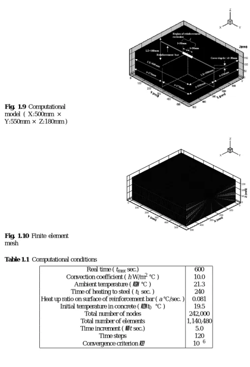
In this study, the computational model shown in Figure 1.9 is employed. The finite element mesh is shown in Figure 1.10. The total number of nodes and elements are 242,000 and 1,140,480 respectively.
The computational conditions are shown in Table 1.1. In addition, the temper- ature boundary condition is given on the surface of the reinforcement bar. The temperature is given until T=240 sec., and the Neumann boundary condition, i.e.
the heat flux is equal to zero, is given on the boundary after T=240 sec. (Equation (1.18)). The boundary condition shown in Equation (1.19) is given on the concrete surface. The observation point is set at the point, X=0.250m, Y=0.275m, Z=0.180m.
The weighting diagonal matrix [Q] is set 1.0 at the observation point, and is set 0.0 at the other points. In addition, the physical constants are shown in Table 1.2. ρ , c and κ denote the density, the specific heat and the thermal conductivity.
φ = a × t + φ (t 0 ) on steel surface in t ∈ [0, t 1 ],
b = 0 on steel surface in t ∈ (t 1 ,t max ], (1.18) b = h × ( φ − φ ∞ ) on concrete surface in t ∈ [0,t max ]. (1.19) In this study, the initial corrosion thickness h and the initial corrosion length of L are set 1.0mm and 100.0mm, and the time history of the temperature obtained by the forward analysis is used as the observed temperature 2 .
1
The iterative computation indicates the computation by the element-by-element conjugate gradi- ent method.
2
In Figures 1.14 and 1.15, the dot line indicates the computational result obtained by the forward
analysis.
Fig. 1.9 Computational model ( X:500mm × Y:550mm × Z:180mm )
Fig. 1.10 Finite element mesh
0 50 100 150
Z(mm)
0 100 200 300 400 500
X (mm) 0
100 200
300 400
500 Y (mm)
X Y
Z
Table 1.1 Computational conditions
Real time ( t
maxsec.) 600
Convection coefficient ( h W/m
2℃ ) 10.0 Ambient temperature ( φ
∞℃ ) 21.3 Time of heating to steel ( t
1sec. ) 240 Heat up ratio on surface of reinforcement bar ( a ℃/sec. ) 0.081
Initial temperature in concrete ( φ (t
0) ℃ ) 19.5
Total number of nodes 242,000
Total number of elements 1,140,480 Time increment ( ∆ t sec.) 5.0
Time steps 120
Convergence criterion ε 10
−6Table 1.2 Physical constants
Concrete Reinforcement bar Reinforcement corrosion ρ (kg/m
3) 2.40 × 10
37.85 × 10
35.30 × 10
3c (J/kg ℃) 1.15 4.70 × 10
−11.20
κ (W/m ℃) 2.70 5.13 × 10
16.97 × 10
−21.4.2 Numerical experiments
If the X-Z plane is represented by the polar coordinate system, a term of the first variation ∂ ∂ J x
∗i
δ x i is formulated as Equation (1.20).
∂ J ∗
∂ x i
δ x i = ∂ J ∗
∂ x δ x + ∂ J ∗
∂ y δ y + ∂ J ∗
∂ z δ z
= ∂ J ∗
∂ y δ y + ( ∂ J ∗
∂ x ∂ x
∂ r + ∂ J ∗
∂ z ∂ z
∂ r
) δ r + ( ∂ J ∗
∂ x ∂ x
∂θ + ∂ J ∗
∂ z ∂ z
∂θ ) δθ
= ∂ J ∗
∂ y δ y + ∂ J ∗
∂ r δ r + ∂ J ∗
∂θ δθ . (1.20)
In Equation (1.20), the variation δθ is equal to zero in case that the corrosion shape is assumed as the concentric circle shape. Therefore, Equation (1.20) is written as Equation (1.21).
∂ J ∗
∂ x i δ x i = ∂ J ∗
∂ y δ y + ∂ J ∗
∂ r δ r
= ∂ J ∗
∂ y δ y + ( ∂ J ∗
∂ x
∂ x
∂ r +
∂ J ∗
∂ z
∂ z
∂ r ) δ r
= ∂ J ∗
∂ y δ y + ( ∂ J ∗
∂ x cos θ + ∂ J ∗
∂ z sin θ ) δ r. (1.21) In this examination, the dependency of the final shape, i.e. the obtained corro- sion shape at the final iteration, for the initial corrosion length is investigated. The initial thickness h is given as 2.0mm, and the initial length L are set 80.0mm(Case 1), 100.0mm(Case 2) and 120.0mm(Case 3) respectively.
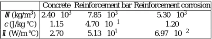
As the computational results, the variation of performance function for each case
is shown in Figure 1.11. It is seen that the value of performance function converges
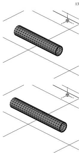
in all cases. The final shape of the reinforcement corrosion for each cases are shown
in Figures 1.12 1.13 and 1.14, and the comparison of volume V , the thickness h and
the length L for the reinforcement corrosion is shown in Table 1.3. In Case 2, it is
found that the obtained corrosion shape at the final iteration could be close to the
target shape (h=1.0mm, L=100.0mm). On the other hand, the final shape could not
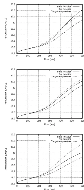
be close to the target shape in Case 1 and 3. In addition, Figures 1.15, 1.16 and 1.17
show the time history of temperature at the observation point for each case. The
solid and the broken and the dot lines denote the computed temperature at the final
iteration, the computed temperature at the first iteration and the target temperature.
It is seen that the computed temperature at the target point is close to the observed temperature in both cases. In this study, it was found that whether the appropriately shape can be obtained depends on the initial shape of the reinforcement corrosion.
According to these results, even if the practical size of reinforcement corrosion is given as the computational condition, it is not usual that the computed temperature is good agreement with the observed temperature. Therefore, if the computation of corrosion shape determination is carried out based on methodology shown in this paper, it is necessary to modify the physical constants such that the computed temperature is agreement with temperature observed by infrared sensor.
0 0.5 1 1.5 2 2.5 3
0 5 10 15 20 25 30 35 40 45 50
Normalized performance function
Number of iterations
Case1 : L=80mm Case2 : L=100mm Case3 : L=120mm
Fig. 1.11 Comparison of variation of performance function
Fig. 1.12 Final shape of reinforcement corrosion (Case 1 : Initial length 80mm)
X Y
Z
Fig. 1.13 Final shape of reinforcement corrosion (Case 2 : Initial length 100mm)
X Y
Z
Fig. 1.14 Final shape of reinforcement corrosion (Case 3 : Initial length 120mm)
X Y
Z
Table 1.3 Comparison of computational results
V(mm
3) h(mm) L(mm)
First iteration (Case 1) 7,513 2.00 80.00
Final iteration (Case 1) 9,251 2.34 84.39
First iteration (Case 2) 9,391 2.00 100.00
Final iteration (Case 2) 4,980 1.26 100.00
First iteration (Case 3) 11,269 2.00 120.00
Final iteration (Case 3) 5,544 1.19 120.00
Target value 4,708 1.00 100.00
Fig. 1.15 Time history of temperature at the observation point (Case 1 : Initial length 80mm)
19.5 19.6 19.7 19.8 19.9 20 20.1 20.2 20.3
0 100 200 300 400 500 600
Temperature (deg C)
Time (sec)
Final iteration 1st iteration Target temperature
Fig. 1.16 Time history of temperature at observation point (Case 2 : Initial length 100mm)
19.5 19.6 19.7 19.8 19.9 20 20.1 20.2 20.3
0 100 200 300 400 500 600
Temperature (deg C)
Time (sec)
Final iteration 1st iteration Target temperature
Fig. 1.17 Time history of temperature at observation point (Case 3 : Initial length 120mm)
19.5 19.6 19.7 19.8 19.9 20 20.1 20.2 20.3
0 100 200 300 400 500 600
Temperature (deg C)
Time (sec)
Final iteration 1st iteration Target temperature