To appear in Engineering Optimization Vol. 00, No. 00, Month 20XX, 1–17

To appear in Engineering Optimization Vol. 00, No. 00, Month 20XX, 1–17

Numerical shape identification of cavity in three dimensions based on thermal non-destructive testing data

T. Kurahashi

, K. Maruoka

and T. Iyama

a

Nagaoka University of Technology, 1603-1 Kamitomiokamachi, Nagaoka, Niigata, Japan;

b

Graduate School of Nagaoka University of Technology, 1603-1 Kamitomiokamachi, Nagaoka, Niigata, Japan;

c

National Institute of Technology, Nagaoka College, 888 Nishikatakai, Nagaoka, Niigata, Japan

(v4.1 released April 2013)

Shape identification analysis is carried out to obtain hitherto unknown defect shapes in a structure, based on the finite element and the adjoint variable methods. In this study, a test piece incorporating a known defect shape was employed to solve the shape identification problem. We also describe the shape identification problem of a cavity in a heated resin test piece made using a 3D printer by employing the temperature pattern observed on the surface of the test piece. The surface temperature of a test piece will not be uniformly distributed if it contains cavities. Practical experiments have confirmed that the characteristic of the temperature distribution depends on the size of the cavity. The thermal physical constants, i.e., the thermal conductivity and the convection coefficient, were identified for a model of the test piece incorporating a cavity based on the experimental data. Shape identification analysis was then carried out. Using numerical analysis, the finite element method was applied to simulate the temperature distribution in the test piece, and the adjoint variable method was employed to identify the cavity’s shape.

Keywords: shape identification analysis; thermal testing method; heat conduction analysis; finite element method; adjoint variable method

1. Introduction

In this paper, we present three dimensional shape identification of defect in a structure based on the finite element and adjoint variable methods using the temperature history on specimen surface. A lot of researches investigate the shape of defect, i.e., cavity, corrosion etc., based on the measurement value on target structures. Kitahara et. al (2002),Yang (2013), Mares (2004), and Hirose (2004) identify the defect shape in concrete using the data of ultrasonic wave. In those researches, the linearized inverse scattering analysis is applied to identify the defect shape, and can be divided into two techniques, the Born and the Kirchhoff inversions. The approximation of using the ultrasonic wave in low and high frequencies is carried out in the Born and Kirchhoff inversions, respectively. It is said that the inner shape of the defect can be accurately obtained in the Born inversion, and, on the other hand, the outside shape of the defect can be accurately obtained, in the Kirchhoff inversion. Conventionally, those methods are employed for two dimensional problems (Blestin, Cohen, and Hagin 1987) three dimensional problems (Yamada et al.

2003; Cohen, Hagin, and Bleistein 1986) and inhomogeneous material problems (Tijhuis

∗Corresponding author. Email: [email protected]

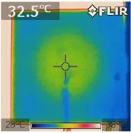
Figure 1. Thermal image

1989). Furthermore, the shape identification of the defect based on the thermal testing (Sahnoun and Belatter 2003; Grys and Minkina 2013) has been proposed, and we focused on this method in this study. Thermal testing is a non-destructive testing method that is used to identify corrosion in structures in the fields of civil and mechanical engineer- ing. It is employed to detect the presence of defects using thermal images obtained by thermography. It has the additional advantage of allowing defect inspection via existing surfaces. Figure 1 shows an example of a thermal image of the top surface of a sample with a cavity that has been heated from its lower surface. The center and edge samples have different temperatures, indicating that the sample has a defect. However, the size and depth of some defects makes them difficult to detect.

Observed temperature by thermal testing methods have been attempted to solve this problem, in which the shape of defect is identified using the temperature based on some numerical methods. For instance, the internal erosion surface shape is estimated based on the extended Kalman filter using the observed temperature on target structure (Tanaka and Ishigami 2006). On the other hand, shape identification analysis based on the finite element and adjoint variable method is also carried out using the observed temperature on concrete surface by the induction heating method (Kurahashi and Oshita 2010a,b).

In the previous study (Kurahashi and Oshita 2010a,b), the shape identification problem of corrosion in concrete is carried out based on data of thermal testing method, and the computation of the identification is carried out under the condition that the corrosion shape is expressed by the cylindrical shape. Actually, the defect shape is arbitrary, it is desired that shape identification is carried out without shape constraint condition. In this study, the shape identification of a cavity whose shape is the ellipsoid body is carried out based on observed data of thermal testing in three dimensions, and some numerical results and remarks are shown in this paper.

2. Experimentation using the nondestructive thermal testing method 2.1 Experimental conditions

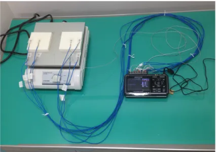
A photo of the experiment is shown in Figure 2, and a drawing of the test piece used

in this study is shown in Figure 3(a). The sample, made of ABS resin, was created

using a 3D printer. A 10 mm-thick test piece with a cavity and an otherwise identical

test piece without a cavity were created. The pair of test pieces (15-mm cavity, no

cavity) were placed on a hotplate and heated for 1200 seconds. The temperature at two

Figure 2. Experimental apparatus

(a) Drawing of the test piece (b) Location of measurement points Figure 3. Observational conditions

observation points on the surface was measured every 10 seconds using a thermocouple.

The observation points were positioned on the surface above where the cavity was thick (Point A) and above where the cavity was thin (Point B) (See Figure 3(b)).

2.2 Observational results

The measured temperature history at Point A and Point B is shown in Figure 4(a) and

(b). The results show that, irrespective of the presence or absence of the cavity, there are

no major differences between the test pieces in the temperature history observed at Point

24 26 28 30 32 34 36 38

0 200 400 600 800 1000 1200

Temperature (deg C)

Time (s)

With cavity Without cavity

(a) A-cavity-15

24 26 28 30 32 34 36 38

0 200 400 600 800 1000 1200

Temperature (deg C)

Time (s)

With cavity Without cavity

(b) B-cavity-15 Figure 4. Observational result using a test piece with a 15-mm cavity

24 26 28 30 32 34 36 38

0 200 400 600 800 1000 1200

Temperature (deg C)

Time (s)

With cavity Without cavity

(a) A-cavity-10

24 26 28 30 32 34 36 38

0 200 400 600 800 1000 1200

Temperature (deg C)

Time (s)

With cavity Without cavity

(b) B-cavity-10 Figure 5. Observational result using a test piece with a 10-mm cavity

B. However, it was confirmed that, at Point A, the temperature of the test piece with a cavity tended to increase faster than the test piece without a cavity. This appears to be due to the influence of convective heat transfer from the air within the cavity. Similar experiments were carried out using a test piece with a 10-mm cavity. The temperature history measured at Points A and B is shown in Figure 5(a) and (b). The results reveal that, at Point A, the change in temperature for the test piece with a 10-mm cavity is smaller than for the test piece with a 15-mm cavity. The thickness of the cavity therefore influences the temperature history at the surface of the test piece.

3. Identification of cavity shape

Shape identification analysis was then carried out using the observational data. We set

the target shape as incorporating a cavity thickness of 15 mm. The initial shape model

is given as incorporating a cavity thickness of 13 mm.

Figure 6. Boundary definition of the test piece

3.1 State equation

Formulation in the shape identification analysis is described below. In this study, the whole domain of the test piece is denoted as Ω. The temperature distribution ϕ therefore satisfies the heat transfer equation shown in Eq. (1).

ρc ϕ ˙ − κϕ

= 0 in Ω (1) For the heat transfer equation, the initial condition and boundary condition are defined as in Eq. (2).

 

 

 



ϕ = ˆ ϕ(t

) in Ω, ϕ = ˆ ϕ on Γ

,

− κϕ

n

= h

(ϕ − ϕ

) on Γ

,

−κϕ

n

= h

(ϕ − ϕ

) on Γ

.

(2)

where ρ, c, κ, n

, h

, h

, ϕ

and ϕ

denote density, specific heat, thermal conduc- tivity, unit normal vector, the convective heat transfer coefficient of the space inside the cavity, the convective heat transfer coefficient of the outside surface, ambient tempera- ture and the temperature inside the cavity. Γ

denotes the lower surface, Γ

denotes the outside surfaces, and Γ

denotes the surface of the cavity (See Figure 6).

3.2 Performance function

To evaluate the computed temperature history, the performance function proposed by Oshita et al. (2009) is applied.

J = 1 2

∫

Γobs

∫

t0

R (ϕ − ϕ

)

dt dΩ (3)

where Γ

, t

, t

, R and ϕ

are measurement region, heating start time, heating

termination time, weight, and observed temperature. The weight R is given 1.0 at the

observation points, otherwise that is given 0.0.

3.3 Lagrangian function

The identification of the shape of the cavity is carried out using inverse analysis, applying the adjoint variable method (Kurahashi and Kawahara 2008; Kurahashi 2010).

The adjoint variable method is one of the minimization technique of the performance function, and is suitable for the inverse problems such that a lot of unknown parameters should be solved. The gradient vector of the performance function with respect to coor- dinates on cavity is obtained by using the temperature difference between computational and the observed values at observation points. In this method, the update of the coordi- nate on cavity surface and the re-evaluation of the temperature difference at observation points are iteratively carried out.

Applying Lagrange multiplier λ, the following Lagrangian function is obtained to mini- mize performance function.

J

= J +

∫

Ω

∫

t0

λ (

ρc ϕ ˙ − κϕ

)

dt dΩ (4)

The first variation, which is a necessary condition for minimizing the Lagrangian func- tion, is shown in Eq. (5)

δJ

= δλ ∂J

∂λ + ∂J

∂ ϕ ˙ δ ϕ ˙ + ∂J

∂ϕ δϕ + δx

∂J

∂x

(5) where x

indicates transplantable nodes. The stationary condition is given as a condi- tion under which each term equals zero. Then first term shows the state equation, second and third term show the adjoint equation.

3.4 Finite element equation

The finite element equation shown in Eq. (6) is derived by adopting a shape function for a four-node tetrahedral element into the state equation to spatially discretize the equation using the Galerkin method. The equations are discretized in time based the Crank-Nicolson method.

ρ

c

[M

] { ϕ ˙

}

+ κ[H

] { ϕ

} = { T

} in Ω

(6) In Equation (6) , [M

], [H

], and { T

} indicate

[M

] =

∫

Ωe

{ Φ

} { Φ

}

dΩ (7)

[H

] =

∫

Ωe

{ Φ

} { Φ

}

dΩ (8)

{ T

} = −

∫

Γ2

q { Φ

} dS −

∫

Γ3

q { Φ

} dS (9)

Where q and S indicate heat flux and boundary surface. Superposing a finite element equation for individual domains, such equation can be represented as Eq. (10)

[A(x

)]

{ ϕ ˙ }

+ [B(x

)] {ϕ} = {C(x

)} (10)

3.5 Adjoint equation

From the stationary condition described above, the adjoint equation and conditions are obtained. The adjoint equation is given by the gradient of the Lagrange function with respect to the temperature ϕ, and the following discretized adjoint equation is derived by the finite element method. The adjoint conditions are also shown below.

{ ∂J

∂ϕ }

= − [A]

{ λ ˙ }

+ [B] { λ } + [R] { ϕ − ϕ

} = { S } in Ω (11)

 

 

 



λ(t

) = 0 in Ω, λ = 0 on Γ

, S = 0 on Γ

, S = 0 on Γ

.

(12)

where [R] and { S } indicate weight diagonal matrix expressed by weight R and reaction vector in the adjoint equation, respectively. These equations manifest themselves as an adjoint problem for calculating λ.

3.6 Gradient vector of the Lagrangian function

The final term in Eq. (5) can be calculated with λ as the following equation.

{ ∂J

∂x

}

= {∫

t0

{ λ }

([ ∂A

∂x

] { ϕ ˙

} +

[ ∂B

∂x

]

{ ϕ } − { ∂C

∂x

})

dt }

in Ω (13)

The nodal position on the cavity of the model is updated with the gradient vector, and followed by recalculation of the state equation. The procedure for inverse analysis (Sakawa and Shindo 1980) is described below.

(1) Set of initial coordinates x

and convergence criterion ϵ.

(2) Computation of state equation.

(3) Computation of performance function J

. (4) Computation of adjoint equation.

(5) Update of coordinate x

based on the computed gradient vector

{

∂xi

} . (l is the number of iterations, W is weighting parameter.)

{ x

}

= {

x

} − [W

]

{

∂J

∂x

}

(6) Checking for convergence; if || x

− x

|| < ϵ ,then stop, else go to step 7.

Figure 7. Computational model

Table 1. Computational condi- tions

Total number of nodes 1460 Total number of elements 5552 Total timetmax, sec 600 Time increment ∆t, sec 10

Time steps 60

convergence criterionϵ 10⁻⁶

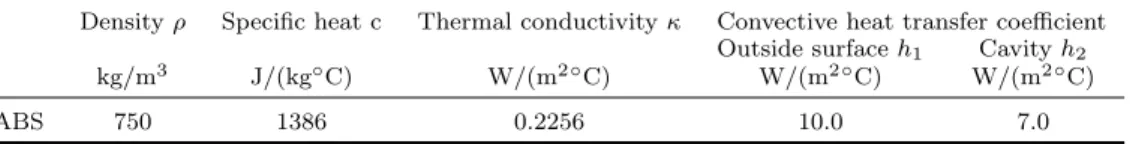
Table 2. Thermal properties of test piece

Densityρ Specific heat c Thermal conductivityκ Convective heat transfer coefficient Outside surfaceh1 Cavityh2

kg/m³ J/(kg^◦C) W/(m^2◦C) W/(m^2◦C) W/(m^2◦C)

ABS 750 1386 0.2256 10.0 7.0

(7) Computation of state equation.

(8) Computation of performance function J

. (9) Updating of weighting parameter W

.

I. if J

< J

, then W

= W

× 0.9, and go to step 4 II. if J

> J

, then W

= W

× 2.0, and go to step 5

3.7 Computational conditions

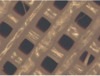
The finite element model of the test piece is shown in Figure 7. The model is composed of four-node tetrahedral elements. The total number of nodes is 1460, and the total number of elements is 5552. The computational conditions are identical to the numerical simulation shown in the previous chapter. Thermal properties for the test piece is given as shown in Table 1 considering the thing which the ABS resin is not filled enough as shown in Figure 8. The observational data at Point A in the previous experimentation is employed as observed temperature. In addition, the time history of temperature on the hotplate and the temperature within the cavity given as boundary conditions are shown in Figure 9(a) and (b).

3.8 Computational results

Figure 10 shows the identified shape of the cavity and Figure 11(a) shows the variation

of normalized performance function per iteration number. The final iteration number is

18, and the performance function is about 0.55 when converting the initial performance

Figure 8. Cross-section of test piece

24 26 28 30 32 34 36 38

0 200 400 600 800 1000 1200

Temperature (deg C)

Time (s)

Hot plate

(a) Hot plate

24 26 28 30 32 34 36 38

0 200 400 600 800 1000 1200

Temperature (deg C)

Time (s)

Cavity

(b) Cavity Figure 9. Time history of temperature at hotplate and cavity surface

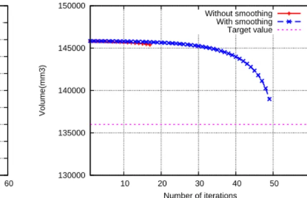
function to 1. However, if the inner surface of the cavity is undulating, the targeted shape assuming a 15 mm-thick cavity cannot be obtained. Neither does the identified volume of the resin region approximate the target value (See Figure 11(b)).

4. The smoothing process

A smoothing process for the gradient vector is adopted to modify the oscillation of the gradient vector with respect to the coordinates on the cavity surface. A Gaussian filter is employed as the smoothing method. The gradient vector is smoothed by assuming the cavity is a two-dimensional surface.

4.1 Gaussian filter

A Gaussian filter is a kind of smoothing filter used for noise suppression in the field of

graphics (Dang and Cahill 1993). In the field of digital filter, some smoothing filter are

proposed such as the averaging filter and the median filter (Imaoka 2000), and the traction

method (Azegami 1994) is frequently employed such that the smoothing equation (Yagi

and Kawahara 2007) is solved. In this study, we focused on the Gaussian filter which

is one of the digital filter. In this smoothing method, we use a Gaussian filter input

with weighted parameters, in which the value of the target nodes is determined by the

values of all the nodes on the same plane. A Gaussian filter provides the additional

advantage that the extent of the smoothing process is adjustable using the parameter

Figure 10. The shape of the cavity at the final iteration(1)

0 0.1 0.2 0.3 0.4 0.5 0.6 0.7 0.8 0.9 1

0 5 10 15 20

Normalized performance function

Number of iterations Performance function

(a) Performance function

130000 135000 140000 145000 150000

0 5 10 15 20

Volume(mm3)

Number of iterations Estimated shape

Target value

(b) Time history of temperature on resin surface at Point B

Figure 11. Computational result(1)

σ, and the computational processes are given as simple vector product. In addition, the shape identification method applying the Gaussian filter has been not approached yet.

The weighting parameter in the Gaussian filter is defined as in the following equation (Ishiwata, Kubota and Shima 2006)

G(x, y) = 1

2πσ

e

2

2σ2

(14)

where x and y are the x-axial distance and the y-axial distance between the target node

and referenced node. The weighting parameter is inversely proportional to distance. The

parameter σ, which in a Gaussian distribution is comparable to variance, determines

the flattening of the distribution. As the summation of the weighting parameter for the

target node becomes 1, we multiply the weighting parameter by the summation. The

weighting parameter for node m to node n is shown in following equation

Figure 12. The shape of the cavity at the final iteration(2)

G

=

1 2πσ²

e

(m)−x(n) )2+(y(m)−y(n) )2 2σ2

∑

1 2πσ

e

(m)−x(n) )2+(y(m)−y(n) )2 2σ2

(15)

where cx is the number of nodes on the surface, x

and y

denote the x-coordinate and the y-coordinate of node m. On the gradient vector

{

∂x^(m)_i

}

, the smoothed gradient vector

{

∂x^(m)_i

′

}

is computed. The calculation formula is represented in the following matrix form.

 

 

 

 

 

 

 



∂J^∗

∂x⁽¹⁾

′

∂J^∗

∂x⁽²⁾

′

∂J^∗

∂x⁽³⁾

′

.. .

∂J^∗

∂x^(cx)

′

 

 

 

 

 

 

 



=



 

 

 

G

G

G

· · · G

G

G

G

· · · G

G

G

G

· · · G

.. . .. . .. . . .. ...

G

G

G

· · · G



 

 

 

 

 

 



 

 

 

∂J^∗

∂x⁽¹⁾

∂J^∗

∂x⁽²⁾

∂J^∗

∂x⁽³⁾

.. .

∂J^∗

∂x^(cx)

 

 

 



 

 

 

(16)

4.2 Shape identification using the Gaussian filter

The parameter σ was given as 20 in computation (Hale 2011), shape identification anal-

ysis was then carried out. The identified shape of the cavity is shown in Figure 12. The

surface of the cavity is smoother than without the smoothing process shown in the previ-

ous section. Variation is apparent in performance function: when using a Gaussian filter,

the greater the number of iterations, the lower the performance function (See Figure

13(a) and Table 3 ). It was also found that the difference in the computed volume of the

resin region at each iteration and the target volume decreases (See Figure 13(b) and Table

4 ). Figure 14 shows the computational temperature history and confirms that applying

the smoothing process causes the computed temperatures to more closely approach the

observed values.

0 0.1 0.2 0.3 0.4 0.5 0.6 0.7 0.8 0.9 1

0 10 20 30 40 50 60

Normalized performance function

Number of iterations Without smoothing

With smoothing

(a) Performance function

130000 135000 140000 145000 150000

10 20 30 40 50 60

Volume(mm3)

Number of iterations Without smoothing

With smoothing Target value

(b) Volume of the resin region Figure 13. Computational result(2)

Table 3. Computational time Without smoothing 4.38(s) With smoothing 10.95(s)

Table 4. Comparison of cavity vol- ume

Without smoothing 145394(mm³) With smoothing 139127(mm³) Target value 136000(mm³)

26 27 28 29 30 31 32

0 100 200 300 400 500 600

Temperature (deg C)

Time (s)

Observed value First iteration Final iteration(without smoothing) Final iteration(with smoothing)

Figure 14. Temperature history

5. The effect of observation point

It is found that identified shape is not good agreement with the target shape, even if the smoothing method is applied. It appears that the computational accuracy increases with increasing the number of observation points.

5.1 Experimentation with multiple observation points

The experimentation using the test piece with a 15-mm cavity was carried out newly. A

lot of 5 observation points including Point A in previous observation are shown in Figure

. Then observational results are shown in Figure and Figure 15(a) The temperature

(a) Observation point

24 26 28 30 32 34 36 38

0 200 400 600 800 1000 1200

Temperature(deg C)

Time(s)

At Point A At Point B At Point C At Point D At Point E

(b) Observational result Figure 15. Experimentation with observation point from A to E

28 30 32 34 36 38 40 42

0 200 400 600 800 1000 1200

Temperature(deg C)

Time(s)

Hot plate

(a) Hot plate

22 24 26 28 30 32 34 36

0 200 400 600 800 1000 1200

Temperature(deg C)

Time(s)

Cavity

(b) Cavity Figure 16. Observational result for hotplate and cavity

observation is carried out by changing the number of observation points as shown in Figure 15(a). The observed temperature is shown in Figures 15(b) and 16.

5.2 Shape identification with multiple observation points

The shape identification analysis is carried out under the three conditions shown below.

Applying time history of temperature at (1) 1 observation point (Point A)

(2) 3 observation points (Point A, Point B and Point E) (3) 5 observation points

The value of the performance function is calculated by using the data at point A in three

computational conditions. The final shape of the cavity in the computational condition

(3) is shown in Figure 17. From this result, it is confirmed that there is no big difference

Figure 17. The shape of the cavity at the final iteration(3)

0 0.1 0.2 0.3 0.4 0.5 0.6 0.7 0.8 0.9 1

0 10 20 30 40 50 60

Normalized performance function

Number of iterations 1 observation points 3 observation points 5 observation points

(a) Performance function

130000 135000 140000 145000 150000

0 10 20 30 40 50 60

Volume(mm3)

Number of iterations 1 observation points 3 observation points 5 observation points Target value

(b) Volume of the resin region Figure 18. Computational result(2)

Table 5. Comparison of cavity volume 1 observation point 138100(mm³) 3 observation points 136723(mm³) 5 observation points 136624(mm³) Target value 136000(mm³)

in each case. In addition, variations of performance function and the volume of resin are shown in Figures 18(a), (b) and Table 5 . Consequently, it is seen that the volume in case of five observation points is close to the target volume. Figure 19 shows comparison of the identified shape and target shape. It is found that the position of the identified shape is upper than that of the target shape.

6. Conclusions

In this study we investigated the shape identification problem of a cavity within a struc-

ture based on the thermal testing method. The test pieces, which incorporated a cavity

with a shape that could be varied, were made using a 3D printer. They were heated from

the underside and their temperature history and distribution was observed. A shape

Figure 19. Comparison of identified shape with target shape

identification analysis was carried out, employing the finite element method for four- node tetrahedral elements and the adjoint variable method. The equations were spatially and temporally discretized using the Galerkin method and the Crank-Nicolson method.

In the identification process, a Gaussian filter was employed to smooth the movement of nodes. The results of our study are shown below.

• When the test pieces were heated from their lower surface, the temperatures of the test piece that included a cavity were higher than those without a cavity at the same observation point and time. The temperature on the face just above the cavity was especially high.

• The temperature history of the test piece during heating varied according to cavity size, with the highest temperatures seen over larger cavities.

• Using a Gaussian filter and smoothing gradient vector, the identified shape of the cavity was smoother than the result calculated without a smoothing process. The calculated temperature also came closer to the observed temperature.

• The accuracy of the identified shape increases in case that the observed data at multi observation points are employed.

It appears that the present method is applicable for the non-destructive testing for defect in reinforced concrete, steel structures and so on. However, the shape of cavity is limited ellipsoidal shape in this study, and it is necessary to extend to identification problems for arbitrary cavity shape in the future.

Acknowledgements

This work was supported by the Program for High Reliable Material Design and Man- ufacturing at Nagaoka University of Technology and a 2015 Grant for Joint Research between Nagaoka College and Nagaoka University of Technology. The computations were mainly carried out using the Fujitsu PRIMERGY CX400 computer facilities at Kyushu University’s Research Institute for Information Technology.

References

Azegami, H. 1994. ”Solution to Domain Optimization Problems” The Japan Society of Mechanical

of Mechanical Engineers (in Japanese) Vol.60, No.574, 165-172

Blesitein, N., Cohen, J. K., and Hagin, F. G. 1987.”Two and one-half dimensional Born inversion with an arbitrary reference” Geophysics Vol.52, No.1, 26-36.

Cohen, J. K., Hagin, F. G., and Bleistein, N. 1986. ”Three dimensional Born inversion with an arbitrary reference” Geophysics Vol.51, No.8, 1552-1558.

Dang, G., and Cahill, L, W. 1993. ”An adaptive Gaussian filter for noise reduction and edge detection” IEEE Nuclear Science Symposium and Medical Imaging Conference Vol.3, 1615- 1619.

Grys, S., and Minkina, W. 2013. ”Filtered thermal contrast technique in thermographic non- destructive testing” AMA Conference 110-115.

Hale, D. 2011. ”Structure-oriented bilateral filtering of seismic images” Research report of Center for Wave Phenomena No.695.

Hirose, S. 2004. ”Quantitative ultrasonic nondestructive evaluation and related technology” Jour- nal of Applied Mechanics (in Japanese) Vol.7, 3-12.

Imaoka, H. 2000. ”Fuzzy Integrals and Smoothing Filters” Japan Society for Fuzzy Theory and Systems Vol.12, No.1, 64-74.

Ishiwata, H., Kubota, H., and Shima, Y. 2012. ”Experimental study on Gaussian filter in restora- tion of error diffused character images” Information Processing Society of Japan (in Japanese) Vol.51, 23-28.

Kitahara, M., Nakahata, K., and Hirose, S. 2002. ”Elastodynamic inversion for shape reconstruc- tion and type classification of flaws” Wave Motion Volume.36, Issue 4, 443-455.

Kurahashi, T. 2010. ”Examination for adjoint boundary conditions in initial water elevation estimation problems” International Journal for Numerical Methods in Fluids Vol.63, 1270- 1295.

Kurahashi, T., and Kawahara, M. 2008. ”Examinations for thermal condition of Lagrange mul- tiplier for heat transfer control problems.” International Journal for Numerical Methods in Engineering Vol.73, 982-1009.

Kurahashi, T., and Oshita, H. 2010a. ”Evaluation of 3D Reinforcement Corrosion Shape in Con- crete Based on Observed Temperature on Concrete Surface.” International Journal of Com- puter Science Vol.4, No.4, 340-351.

Kurahashi, T., and Oshita, H. 2010b. ”Shape Determination of 3-D Reinforcement corrosion in Concrete Based on Observed Temperature on Concrete Surface.” Computers and Concrete Vol.7, No.1, 63-81.

Mares, P. 2004. ”Simulation as a Support for Ultrasonic Testing” Journal of Modern Physics Vol.5, 1167-1172.

Oshita, H., Horie, H., Nagasaka, S., Taniguchi, O., and Yoshikawa, S. 2009. ”Nondestructive evaluation of corrosion in reinforced concrete by thermal behavior on concrete due to electro- magnetic heating” Journal of Japan Society of Civil Enginerrs E (in Japanese) Vol.65, No.1, 76-92.

Sahnoun, S., and Belatter, S. 2003. ”Thermal non destructive testing study of a circular defect in plane structure” NDT.net Vol.8, No.08.

Sakawa, Y., and Shindo, Y. 1980. ”On global convergence of an algorithm for optimal control”

IEEE Transactions on Automatic Control Vol.25, 1149-1153.

Tanaka, M., and Ishigami, H. 2006. ”Estimation of Internal Erosion Surface Shape in Power- Plant Pipelines by Measuring Temperature on External Surface ( Application of BEM and Filter Theory)” The Japan Society of Mechanical of Mechanical Engineers Vol.19, No.06-9, 421-422.

Tijhuis, A. G. 1989. ”Born-Type Reconstruction of Material Parameters of an Inhomogeneous , Lossy Dielectric Slab from reflected-Field Data” Wave Motion Vol.11, Issue 2, 151-173.

Wang, S., Li, W., Wang, Y., Jiang, Y., Jiang, S., and Zhao, R. 2012. ”An improved Difference of Gaussian Filter in Face Recognition” Journal of Micromechanics and Microengineering Vol.7, No.6, 429-433.

Yagi, H., and Kawahara, M. 2007. ”Optimal shape determination of a body located in incom- pressible viscous fluid flow” Computer methods In applied mechanics and engineering Vol.196, Issues 49-52, 5084-5091.

Yamada, M., Mkurakami, K., Nakahata, K., and Kitahara, M. 2003. ”Three Dimensional Born

and Kirchhoff Inversions for Shape Reconstruction of Defects” Review of Quantitative Nonde-

structive Evaluation Vol.22, 734-741.

Yang, Y. 2013. ”Ultrasonic testing of the application of the concrete defects” International Con-

ference on Education Technology and Management Science 319-321.