Shape Optimization using GA with Stress-based Crossover

Transactions of JSCES, Paper No.20090002

Shape Optimization using GA with Stress-based Crossover

Cuimin LI

, Tomoyuki HIROYASU

, Mitsunori MIKI

1

Graduate School of Engineering, Doshisha Univ.( 610-0321, Kyotanabe)

2

Life and Medical Sciences Department, Doshisha Univ. ( 610-0321, Kyotanabe)

3

Sciences and Engineering Department, Doshisha Univ. ( 610-0321, Kyotanabe)

In this paper, genetic algorithm with a stress-based crossover is improved to solve structural shape optimization problems. The design domain is well divided by finite element method.

According to one initial topology, the boundary profile elements and the neighboring outside elements, which are design variables, are randomly set to “0” or “1” to generate the initial population. To keep the shape deforming gradually, a logical “OR” operation is applied on each child structure and a “mask” structure. Moreover, the material weight of child is adjusted dynamically. Three experiments were performed to verify the effectiveness of improved SX for structural shape optimization.

Key Words: Improved Stress-based Crossover, Stress-based Crossover, Genetic Algorithm,

Shape Optimization, Structure Optimization

1. Introduction

Shape optimization problems consist of finding the best profile of a structural system, which improves its mechanical behavior and minimizes some properties of that structure. The main approaches to shape optimiza- tion include the basis vector method and traction method

(1, 2)

, evolutionary structural optimization (ESO)

, homogenization-based methods

, and SIMP method

. Recently, there has been researches regarding the appli- cation of genetic algorithms (GAs)

for structure op- timization because they do not require sensitivity anal- ysis during optimization. In this paper, we will discuss application of GAs to shape optimization.

Traditionally, continuum shape is defined by the ori- ented boundary curves or boundary surfaces of the body.

Tanie and Kita

use GAs to optimize the shape of continuum 2D structures through B-spline. Woon et al.

investigated alternative encodings of GAs for con-

∗ 2008 11 05 , 2009 01 07

, 2009 01 28 , c2009 . Manuscript received, November 05, 2008; final revision, Jan- uary 07, 2009; published, January 28, 2009. Copyright c2009 by the Japan Society for Computational Engineering and Sci- ence.

tinuum shape optimization using the actual coordinates of boundary nodes. The boundary is represented by b- spline functions, circles, and polylines, the control points of which constitute the parameters that govern the shape of the structure. This requires a large number of design variables and it is also difficult to maintain an adequate finite/boundary element mesh during the optimization process. Moreover, the mesh file should be refreshed once the node coordination changes.

Another approach of GAs to structure shape optimiza- tion involves discretising the initial design domain into a mesh of elements, whereby each element is associated with a string bit

. The material constants at the mesh, such as the density and Young

s modulus, are taken as the design variables. The mesh with material is set to “1” and that without material is set to “0.” In this case, the finite element method is usually employed for estimating the objective functions and the constraint con- ditions. By this method, detailed well-designed domain division is necessary to avoid a zigzag-shaped boundary.

Previous research

verified that stress-based crossover

(SX)

can perform topology optimization even with

a roughly designed domain division. Then, shape opti-

mization should be used to smooth the structure bound-

ary profile. In this paper, SX is improved to solve shape optimization problem. In the present scheme, shape opti- mization starts from an initial topology obtained by SX.

Three stress and displacement constrained experiments are performed to show the effectiveness of our improved stress-based crossover (iSX).

2. Shape Optimization using Stress-based Crossover

2.1 Design Variables and Chromosome Rep- resentation Before shape optimization, topology optimization is performed using SX with rough design do- main division. After that, shape optimization is applied to further optimize the structure profile. Here, we will present an example to explain the design variables. First, the design domain inside the rectangle as shown in Fig.1- (a) is further divided into small meshes. Each structure is taken as one chromosome. The material distribution in each mesh is taken as one gene on the chromosome with

“0” representing void and “1” representing material. The black part of Fig.1-(b) is the profile meshes of Fig.1-(a).

The grey part of Fig.1-(b) is the “0” neighboring meshes of profile meshes of Fig.1-(a). These meshes in Fig.1-(b) are design variables. During GA evolution, the design variables vary with the structure profile.

(a) initial structure (b) parameter elements

(c) an example individual (d) mask individual p

Fig.1 Preparation for Shape Optimization

2.2 Population Initialization For shape op- timization, the initial population is generated from the initial structure by randomly setting the design variables to “0” or “1.”. One example individual is shown in Fig.1- (c). In order to keep the same topology during shape optimization, a mask individual as shown in Fig.1-(d), which is the inner solid elements of Fig.1-(a), is saved. A logic “OR” operation is applied on the mask individual and each child individual.

2.3 Procedures of iSX In this section, we will introduce the procedures of iSX for structural shape op- timization. The details of step 3 are illustrated in Fig.2.

Firstly, the nomenclatures are explained.

•

initial: the initial structure as Fig.1-(a)

•

p

: the profile elements of structure, the black part as Fig.1-(b)

•

p

: the neighboring “0” element of p

, the grey part as Fig.1-(b)

•

p

: the inner solid elements as Fig.1-(d)

•

p

: the elements of p

and p

•

p.weight: the “1” number of individual p

•

p.stress[k]: element stress of individual p, k = 1 . . . n, n is equal to the chromosome length

•

child

.ability[k]: ability value of each gene of child individual child

, k=1 . . . n

•

P (t) =

(t)|i = 1 . . . N

of generation - t, N is population size

•

P

(t) =

(t)|i = 1 . . . N}: children pop- ulation

Procedures of iSX for shape optimization (1) Randomly generate the initial population P (t) from

structure-initial, save parent

.

(2) Finite element analysis for each structure to calcu- late element equivalent stress

(3) SX operation to generate offsprings population P

(t).

Applying the following steps to generate child in- dividuals

(3-1) For each individual parent

, randomly se- lect the other individual parent

from P (t) , here i

j

(3-2) Sum the element stress with same element number as formula (1)

child

.ability[k] = parent

.stress[k]

+parent

.stress[k]

(1) (3-3) Sort child

.ability[k] from large to small (3-4) The front m elements with large ability value

is set to “1”. Others will be set “0”. The def- inition of m will be discussed in the section 2.5

(3-5) Logic “OR” operation for child individual

child

and parent

to recover the changed

elements that are not parameter elements

After step (3-1)-(3-4), many other elements may

have their gene values changed. Therefore, step

(3-5) is used to recover these genes. It should be

noted that only one child is generated after the

above operations. Apply the above steps on P (t)

to generate children population P

(t).

6.0 5.9 4.4 1.5

9.0 7.9 8.4 6.5 (3-1)

parent (t).gene[k]

parent (t).mask[k]

child (t).gene[k]

parent (t).stress[k]

15.0 13.8 12.8

8.0

child (t).ability[k]

parent (t).gene[k] parent (t).stress[k]

P(t)

P'(t)

(3-3)

(3-4)

(3-5) (3-2)

... 2.2 ... 8.0 ... 20.9

m n-m

logical "OR"

i i i

i

i

j j

Fig.2 Detail of step (3) of iSX Procedures

(4) Finite element analysis for children population P

(t) (5) Fitness evaluation for P

(t) and save the best indi-

vidual

(6) If termination, go to (7); else, generate child

from P

(t). Randomly reset “0” or “1” to generate the next population P(t + 1), go to (2)

(7) Finished

Shape optimization starts from an initial structure.

Initially, the profile elements of the structure (width=1) and the neighbor “0 elements (width=1) are set param- eters and all the initial individuals have the same mask structure. After the first generation, the parameters ele- ments and mask structures are reset again for each indi- vidual. From the second generation, each individual has different parameters and mask structure. The parameter elements become more and more and the mask structure becomes thin.

2.4 Multi-constrained Problem Description and Fitness Definition

In this paper, three experiment problems with stress and displacement constraints were adopted to show the effectiveness of iSX. The optimization problem is shown in formula (2).

min.f(X) =

n

X

i=1

x

, x

1}

subject to : Stress

< Stress

Displacement < Displacement

(2)

For GAs, the fitness function definition that deter- mines which individuals will be preserved in the next generation is very important. A penalty function is used for multi-constrained problems. The fitness function for feasible individuals is shown in formula (3).

f itness =

n

X

i=1

x

+ Stress

Stress

+ Displacement Displacement

(3)

The first term represents the objective function; the second and third terms are penalty functions. For fea- sible individuals the last two terms are less than 1 so that the fitness function focuses on optimize the objec- tive function. For infeasible individuals, the first term is replaced by a constant that is larger than the objective value of any feasible individual. That is, any feasible in- dividual is preferred over any infeasible individual. For infeasible individuals, those with smaller constraint vio- lations are preferred.

2.5 Violation Handling Strategy

We construct a violation handling strategy for infea- sible individuals during iSX optimization. In iSX proce- dure step (3-4), the definition of m is different for feasible and infeasible parents. In this paper, m is defined as for- mula 4, where r is a uniform random number between 0 and 1. For infeasible parent individuals, the weight of child individual is defined as the same as that of the par- ent. If the parent is a feasible individual, the “1” number in the child individuals will reduce gradually. However, the reduction of “1” cannot be greater than half of the profile element number. It means once a feasible indi- vidual is searched out, the weight of child individual will decrease gradually. From this point, the iSX operator is similar to ESO method that is effective for local searches.

m =

(

p

.weight, if p

is infeasible

p

.weight + p

.weight

r

0.5, if p

is feasible

(4)

3. Experiment

In this section, three experiments are performed to show the effectiveness of iSX for shape optimization.

•

Example a:

The first example is a single-load Michell MBB problem. The design domain is 10000×5000 mm as shown in Fig.3. The two corners at the bottom are fixed and a downward concentrated load F = 1000 N is applied at mid-span on the lower frame. The half design domain is divided into 50

50 meshes.

The material to occupy the design domain is cho- sen as steel with modulus of elasticity of 210 GPa and Poisson

s ratio of 0.3. Due to symmetry, only half of the structure is analyzed. The objective function is to minimize weight resulting in maxi- mal stress less than 0.25 Pa and displacement of loading point less than 2.0

10

mm.

1000mm

500mm

F=1000N

Fig.3 Michell MBB Problem

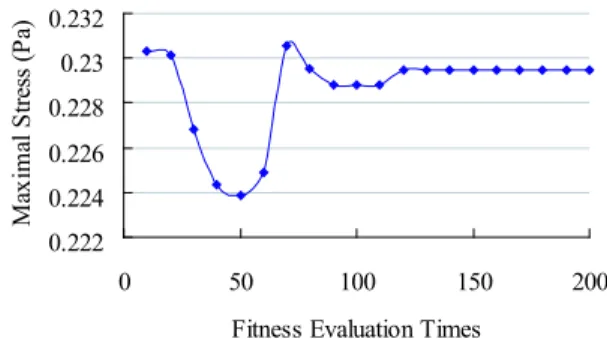
The initial shape and some iteration results shown in Fig.4 illustrate that the structure shape becomes smooth. The weight, maximal stress and displace- ment evolution history are shown in Fig.5, Fig.6 and Fig.7 respectively. The finite element anal- ysis results of initial shape and final shape are compared in Table 1. The maximal stress and displacement iteration histories demonstrate the global search ability of iSX for shape optimization.

initial shape generation=2 generation=6

generation=10 final shape Fig.4 Shape Variation of Michell Problem

•

Example b:

This example is also an MBB beam problem. As a

0 0.2 0.4 0.6 0.8

0 50 100 150 200

Fitness Evaluation Times

Weight (%)

Fig.5 Weight Iteration History of Michell Problem

0.222 0.224 0.226 0.228 0.23 0.232

0 50 100 150 200

Fitness Evaluation Times

Maximal Stress (Pa)

Fig.6 Maximal Stress Iteration History of Michell Problem

1.0E-09 1.2E-09 1.4E-09 1.6E-09 1.8E-09 2.0E-09 2.2E-09

0 50 100 150 200

Fitness Evaluation Times

Displacement (mm)

Fig. 7 Displacement Iteration History of Michell Problem

Table 1 Structure Analysis Results of Initial Struc- ture and Final Structure

Index Weight Stress

Displacement (%) (Pa) (mm) ×10

Initial Shape 82.0 0.228 1 . 72

Final Shape 18.6 0.229 1 . 97

benchmark example, it has previously been stud- ied extensively by applying homogenization meth- ods and traditional boundary variation methods.

As shown in Fig.8, a simply supported beam has a span L=240 mm, height H=40 mm, and thickness T=1 mm, with a concentrated load P=1000 N ap- plied at mid-span. During the computing process, due to symmetry, only half of the structure is mod- eled using 120×40 hex quadrilateral elements. The objective function is to minimize weight resulting in maximal stress less than 3000 Pa and displace- ment of loading point less than 2.5

10

mm.

240mm

40mm F=1000N

(a) mbb-beam

120mm

40mm F=1000N

(b) half of mbb-beam

Fig.8 Michell MBB Problem

For this problem, two experiments were performed with the initial structures shown in Fig.9 and Fig.11.

The results are shown in Fig.10 and Fig.12, respec- tively. The structure properties are compared in Table 2 and Table 3.

Fig.9 Initial Shape of Experiment (1)

Fig.10 Final Shape of Experiment (1) Table 2 Structure Properties of Expeirment (1)

Index Weight Stress

Displacement (%) 10

(Pa) 10

(mm)

Fig.9 52.00 2.516 2.207

Fig.10 41.41 2.520 2.488

Fig.11 Initial Shape of Experiment (2)

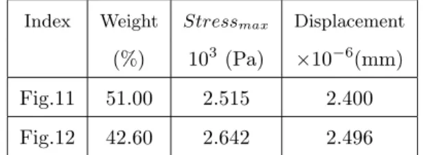
Fig.12 Final Shape of Experiment (2) Table 3 Structure Properties of Experiment (2)

Index Weight Stress

Displacement (%) 10

(Pa) × 10

(mm) Fig.11 51.00 2.515 2.400 Fig.12 42.60 2.642 2.496

•

Example c:

This is a multiple load problem. As shown in Fig.13, the rectangular design domain is 12 m in length and 6 m in height, the bottom left corner is fixed, and the bottom right corner is constrained as rolling condition. Three forces are applied at the bottom at equally spaced points with P1=300 N, P2=P3=150 N . During the optimization process, only the right half is analyzed and discretized by 60×60 hexahedral elements. The Young

s modu- lus for “1” material is 200 MPa and Poisson

s ratio is 0.3. The Young

s modulus for “0” material is 1 MPa and Poisson

s ratio is 0.3.

The initial shape, variations of generations 2, 4 , 6, 8 and the final shape are shown in Fig.14.

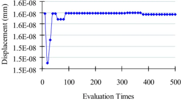
The properties of the initial and final structures are compared in Table 4. The weight, displace- ment, maximal stress iteration histories are shown in Fig.15, Fig.16 and Fig.17.

P1

P2 P3

Fig.13 Multi-load Beam Problem

Table 4 Structure Properties of Initial Shape and Final Shape of Multi-load Beam Problem

Index Weight Stress

Displacement (%) (Pa) × 10

(mm) Initial Shape 56.00 1.137 1.681

Final Shape 37.61 1.136 1.596

iteration=2

initial shape iteration=4

iteration=6 iteration=8 final shape

Fig. 14 Iteration History Results of Multi-Load Beam Problem

0.35 0.4 0.45 0.5 0.55

0 100 200 300 400 500

Evaluation Times

Weight (%)

Fig. 15 Weight Iteration History of Multi-Load Beam Problem

1.5E-08 1.5E-08 1.5E-08 1.6E-08 1.6E-08 1.6E-08 1.6E-08

0 100 200 300 400 500

Evaluation Times

Displacement (mm)

Fig. 16 Displacement Iteration History of Multi- Load Beam Problem

1.1355 1.136 1.1365 1.137 1.1375 1.138 1.1385

0 100 200 300 400 500

Evaluation Times

Maximal Stress (Pa)

Fig.17 Maximal Stress Iteration History of Multi- Load Beam Problem

Fig.14 shows that the general shape is determined on generation 6. Subsequently, the objective func- tion is further optimized according to the fitness function definition. Due to the global search abil- ity of iSX, a more optimal solution is searched out but the topology is changed.

4. Conclusion

This paper introduced an improved stress-based crossover for shape optimization. This operator begins from an ini- tial topology with the design domain being well divided by fixed meshes. During the evolution process, the pro- file elements of the structure, which are design variables, varies gradually. A logical “OR” operation is applied on a mask structure and each new child structure to guarantee the structure shape optimized gradually. The “1” num- ber of child individuals is adjusted dynamically. Three experiments show the effectiveness of iSX for structural shape optimization. Comparison of the initial and final structures demonstrated the ability of iSX to produce optimal shapes based on stress and displacement criteria through a sequence of steps based on sets of locally opti- mized structure profile elements. The method was shown to be able to identify and remove material that effectively increases the structure’s fitness as well as add material to gradually contribute to the shape profile. Moreover, by the dynamic adjustment of the “1” number in child individuals and fitness function definition, iSX always at- tempts to perform the optimization process until termi- nation.

Reference

(1) Azegami Hideyuki., A solution to domain optimiza- tion problems, Transactions of the Japan Society of Mechanical Engineers. A Vol. 60, No.574(19940625) pp.1479-1486, 1994.

(2) Azegami Hideyuki., A SMOOTHING METHOD

FOR SHAPE OPTIMIZATION: TRACTION

METHOD USING THE ROBIN CONDITION, International Journal of Computational Methods, Vol. 3, No. 1, pp.21-33, 2006.

(3) Xie, Y.M., Steven, G.P., A simple evolutionary pro- cedure for structural optimization, Comput. Struct, Vol.49, pp.885-896, 1993.

(4) Xie, Y.M., Steven, G.P. , Evolutionary Structural Optimization,. London: Springer, 1997.

(5) Bendsoe, M.P. and Kikuchi, N., Generating optimal

topologies in structural design using a homogeniza-

tion method, Comput. Methods. Appl. Mech. Engre.,

Vol.71, pp.197-224, 1988.

(6) Zhou, M.; Rozvany, G.I.N. , The COC algo- rithm, part II: topological, geometrical and gener- alized shape optimization, Comput. Methods Appl.

Mech. Eng., Vol.89, pp.309-336, 1991.

(7) Rozvany, G.I.N.; Zhou, M.; Birker, T. , Generalized shape optimization without homogenization., Struct.

Optim., Vol.4, pp.250-252, 1992.

(8) Holland, J.H., Adaptations in Natural and Artificial Systems, London: MIT Press, 1975.

(9) Goldberg, D.E. , Genetic Algorithms in Search, Op- timization and Machine Learning, Mass.: Addison- Wesley, 1989.

(10) TANIE HISASHI and KITA EISUKE, Topology and Shape Optimization of Continuum Structures by Genetic Algorithm, Transactions of the Japan Society of Mechanical Engineers. A, Vol.65, NO.634, pp.1420-1426, 1999.

(11) S.Y. Woon, O.M. Querin and G.P. Steven, On im- proving the GA step-wise shape optimization method through the application of the Fixed Grid FEA paradigm , Structural and Multidisciplinary Opti- mization, Volume 25, Number4, pp.270-278, 2003.

(12) Schoenauer, M., Shape representation for evolu- tionary optimization and identification in structural mechanics, Genetic Algorithms in Engineering and Computer Science, pp. 371-396. West Sussex: Wiley, 1995.

(13) Chapman, C.D.; Jakiela, M.J., Genetic algorithm based structural design with compliance and topol- ogy simplification considerations, J. Mech. Design.

Vol.118, pp.89-98, 1996.

(14) Li. C., Hiroyasu, T., Miki M., Parameters Dis- cussion of SX for Structural Topology Optimization, Transactions of JSCES, submitted.

(15) Li. C., Hiroyasu, T., Miki M., Stress-Based

Crossover Operator for Structural Topology Opti-

mization, Journal of Computational Science and

Technology Vol. 2, No. 1, pp.46–55, 2008.