Shape optimization analysis for thermal elastic deformation problems in three dimensions based on the adjoint variable and the finite element methods

(1)

y rC o

E024

r h r1 0

p 1 tg

Shape optimization analysis for thermal elastic deformation problems in three dimensions based on the adjoint variable and the finite element methods

*1 *2 *3

Satoshi HIROSE

^*1

, Takahiko KURAHASHI

^*2

and Eiji KATAMINE

^*3

*1

Nagaoka University of Technology, Department of Mechanical Engineering

Abstract

In the field of shape design of machine tools and electronic devices with thermal deformations, shape optimization of thermal elastic fields coupled with thermal conduction and elastic fields is becoming more and more important due to the increasing demand for higher performance. In this paper, we formulate the shape optimization problem for maximizing the stiffness or controlling the displacement in a three-dimensional unsteady thermal elastic field using the adjoint variable and the Lagrange multiplier methods, and theoretically derive the shape gradient function as the sensitivity for updating the shape. The traction method was applied based on the derived shape gradient function, and the validity of the method was confirmed by using the numerical analysis program based on the FreeFEM.

Key Words : Shape optimization , Shape identification , Finite element method ,Adjoint variable method , Thermal

elastic fields

1.

1

(1)

(2) (3)

3

2

0

(4)(5)

FreeFEM

⁽⁶⁾⁽⁷⁾

2.

r1 0 g 2

2 1

!

1

*1 940-2188 1603-1

*2 940-2188 1603-1

*3 501-0495 2236-2

E-mail: [email protected]

(2)

! =

_!^!^! _!

!

_!"#$

!

_!"

! − !

_!

!

_!"

(!

_!

) + !

_!

!

_!

!Ω +

_!

!

_!

!

_!

!

_!

!Γ

!

!" 1

!_!"(!_!)=^!

!(!_!,!+!_!,!)

2

!_! ! !_! !=0 !_!"#$ !_!"

!_! ! !_! ! !_! !

!_! !_! Ω Γ 3

!_!

1 0

∙ _,!=!(∙)/!!_!

2 2

3 ~ 4

!

−

!!

_,!!−!=0

in

!∈ !_!,!_!

in

Ω

3 !

_!"#$

!

_!",!(!_!)−!_!"(!−!_!)_,! +!_!=0

in

!∈ !_!,!_!

in

Ω

4

! ! 3 ∙ =!(∙)/!"

2 3

i

5 ~ 11

!=! at !=!_!

in

Ω

5

!=! in !∈ !_!,!_!

on

Γ_!

6

!=!=−!!_,!!_!

in

!∈ !_!,!_!

on

Γ_!

7

!=ℎ !−!_! =−!!_,!!_!

in

!∈ !_!,!_!

on

Γ_!

8

!_!=!_!

in

!∈ !_!,!_!

in

Ω

9

!_!=!_!

in

!∈ !_!,!_!

on

Γ_!

10

!_!=

!

_!"#$

!

_!"(!_!)−!_!"(!−!_!) !_!

in

!∈ !_!,!_!

on

Γ_!

11

∙ !_! ! ℎ !_! 3 !

Γ_! Γ_! Γ_! Γ_! Γ_! 3

Dirichlet

Neumann Robin Dirichlet

Neumann

2 4

t 2

!^∗ ,!_!^∗ !

Lagrange

!^∗

12

!^∗=!+ _!^!^! _! !^∗

!

−

!!

_,!!−!

! !Ω!"+ _!^!^! _! !_!^∗

!

_!"#$

!

_!",!(!_!)−!_!"(!−!_!)_,! +!_!

! !Ω!"

12

!^∗ !_!^∗

Lagrange

!!^∗

13 ~ 20

!^∗+!!_,!!^∗ −!_!"#$!_!"!_!"(!_!)−!_!"#$!_!"!_!"(!_!^∗)=0

in

!∈ !_!,!_!

in

Ω

13

!_!"#$!_!",!(!_!^∗)−!_!"#$!_!"(!−!_!)_,!+!_!=0

in

!∈ !_!,!_!

in

Ω

14

!^∗=0 at !=!_!

in

Ω

15

!_!^∗=0

at

!=!_!

in

Ω

16

!^∗=0 in !∈ !_!,!_!

on

Γ_!

17

!_!^∗=0 in !∈ !_!,!_!

on

Γ_!

18

!_!^∗=!_!^∗= !_!"#$!_!"(!−!_!)−2!_!"#$!_!"(!_!^∗) !_!

in

!∈ !_!,!_!

on

Γ_!

19

(3)

!^∗=!^∗= !_!"#$!_!"!_!^∗−!!_,!^∗ !_!

in

!∈ !_!,!_!

on

Γ_! and Γ_!

20

Γ!"#$%&

Lagrange

!_!

21

!_!^∗!!_!

!

!_!

!_! !Γ!"+ _!^!^! _! !^∗!"

! !Γ!"

= _! !_!^∗!!_!

!!!_!

!_!

!_! !Γ!"+ _! !_!^∗!_!,!!!_!

!"#$%&

!_!

!_! !Γ!"+ _! !^∗!"

!!!_!!!_!

!_!

!_! !Γ!"+ _! !^∗!_,!!!_!

!"#$%&

!_!

!_! !Γ!"

= _! !_!^∗!!_!

!!!_!

!_!

!_! !Γ!"+ _! !^∗!"

!!!_!!!_!

!_!

!_! !Γ!"+ _! !_!!!_!

!"#$%& !Γ

21

!_! !_!^∗

22

!_!^∗ !

!

!_!^!!! =!_!^! −!!_!^∗^!

22 2 5

Step 1

Step 2

!=!_! !=!_! ! !_!

Step 3 23

!^! −!^!!! !^! <!

23 Step 4 Step 2

! !_! !=!_! !=!_!

!^∗ !_!^∗

Step 5

!_!

Step 6 Step 2

3.

r1 0 2

3 1

!

24

!= _!^!^! _! !_!(!_!−!!(!"#$%!))^!!Γ

! !"

24

!_! !!(!"#$%!) ! !_!

1 0

3 2

t 2

!^∗ ,!_!^∗ !

Lagrange

!^∗

25

!^∗=!+ _!^!^! _! !^∗

!

−

!!

_,!!−!

! !Ω!"+ _!^!^! _! !_!^∗

!

_!"#$

!

_!",!(!_!)−!_!"(!−!_!)_,! +!_!

! !Ω!"

25 Lagrange

!!^∗

26 ~ 33

!^∗+!!_,!!^∗ −!_!"#$!_!"!_!,!^∗ =0

in

!∈ !_!,!_!

in

Ω

26

!_!"#$!_!",!(!_!^∗)+ _!^!^! _! 2!_!(!_!−!!(!"#$%!))!Γ!"

! =0

in

!∈ !_!,!_!

in

Ω

27

!^∗=0 at !=!_!

in

Ω

28

!_!^∗=0

at

!=!_!

in

Ω

29

!^∗=0 in !∈ !_!,!_!

on

Γ_!

30

(4)

!_!^∗=0 in !∈ !_!,!_!

on

Γ_!

31

!_!^∗=!_!^∗= −2!!_!"(!_!^∗) !_!

in

!∈ !_!,!_!

on

Γ_!

32

!^∗=!^∗= !_!"#$!_!"!_!^∗−2!!_,!^∗ !_!

in

!∈ !_!,!_!

on

Γ_! and Γ_!

33

Γ!"#$%&

Lagrange

!_!

21

22 3 3

Step 1

Step 2

!=!_! !=!_! ! !_!

!!(!"#$%!)

Step 3

Step 4

!=!_! !=!_! ! !_!

Step 5 23

Step 6 Step 4

! !_! !=!_! !=!_!

!^∗ !_!^∗

Step 7

!_!

Step 8 Step 4

4. 4 1

1 0.5[GPa] 0.3[-]

11.7×10^!![1/K] !=100[W/m∙

K] Γ_! !=303[K]

Γ_! ℎ=300[W/m^!∙K] !_! =273[K]

Γ_! Γ!"#$%&

!_!=100[kN/m^!] !

!_!=0[s] !_!=1.5×10^!![s] !"=1.5×10^!![s]

102570 20988

Γ_! !_!

0.98 ( a) 3D Representation (b) Boundary condition

Figure 1 Numerical calculation model.

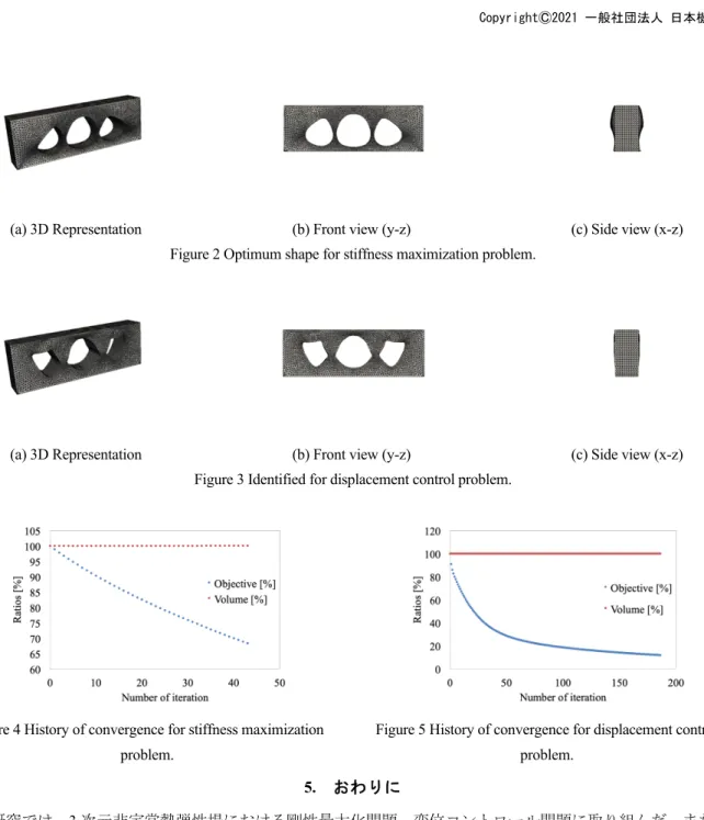
4 2

2 5 2 3

4 5 100

(5)

y rC o

(a) 3D Representation (b) Front view (y-z) (c) Side view (x-z)

Figure 2 Optimum shape for stiffness maximization problem.

(a) 3D Representation (b) Front view (y-z) (c) Side view (x-z)

Figure 3 Identified for displacement control problem.

Figure 4 History of convergence for stiffness maximization problem.

Figure 5 History of convergence for displacement control problem.

5.

1

3 (1) “ ” 77-783

C(2011-11) 4015-4023.

(2) “ ” 83-845 (2017-1)

DOI:10.1299/transjsme.16-00490 13pages.

(3) E. Katamine H. Azegami and M. Hirai “Solution of Shape Identification Problem on Thermoelastic Solids”, International Joumal of Computational Methods Vol.3 No.3(2006-9) 279-293