FLOW FIELD ESTIMATION IN OPEN CHANNEL BASED ON KALMAN FILTER FINITE ELEMENT METHOD

Crete Island, Greece, 5–10 June 2016

FLOW FIELD ESTIMATION IN OPEN CHANNEL BASED ON KALMAN FILTER FINITE ELEMENT METHOD

T. Yoshiara

, T.Kurahashi

, Y.Kobayashi

and T.Eto

1

Graduate school of Nagaoka University of Technology, 1603-1 Kamitomioka, Nagaoka, Niigata, 940-2188, Japan.

e-mail: [email protected]

2

Department of Mechanical Engineering, Nagaoka University of Technology, 1603-1 Kamitomioka, Nagaoka, Niigata, 940-2188, Japan.

e-mail: [email protected]

3

Department of Mechanical Engineering, Nagaoka University of Technology, 1603-1 Kamitomioka, Nagaoka, Niigata, 940-2188, Japan.

e-mail: [email protected]

4

National Institute of Technology Nagaoka college, 888 Nishikatakai, Nagaoka, Niigata, 940-8532, Japan.

e-mail: [email protected]

Keywords: Finite element method, Kalman filter theory, Estimation of flow field

Abstract. The Kalman filter developed by R. E. Kalman and R. S. Bucy is states estimation theory in the target domain and has been employed in various field of engineering. In general, observation data in any system include observation noise and the computational model in- cludes system noise. The finite element equation is applied to derive the state transition ma- trix in the system equation of the Kalman filter. We can estimate state values after the time progress of spatial models. On the other hand, tidal power generation has the potential to contribute significantly as one of the clean energy. In tidal power generation, propellers of generator are rotated by tidal current and tidal power is converted to electric energy. There- fore, the generator should be placed in the fast point of tidal current to produce more electric energy. Thus, we focused on the flow field estimation using the observation data at limited observation points to find out the fast point of tidal current. As the fundamental study, the es- timation of the flow field in open channel is carried out based on the finite element method and the Kalman filter theory. As the governing equation, the shallow water equations are em- ployed, and the finite element and the selective lumping methods are applied to discretize the governing equations in space and time, respectively. The estimation of the distribution of the velocity vector and the water elevation is carried out by using the discretized equation. The open channel model is employed in the numerical experiment, and some examinations are carried out by changing the observation variables, number and position of observation points.

In addition, numerical experiments using practical observed values are carried out.

tions are carried out by changing the observation variables, number and position of observa- tion points.

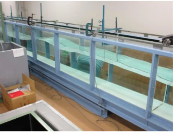
Figure 1: Open channel.

2 DISCRETIZATION OF GOVERNING EQUATIONS

The shallow water equations are used as a governing equations, which is represented as equation (1) and (2) in the two-dimensional plane. u ,  , g , and h are flow velocity, water elevation from the average water depth, the gravitational acceleration and water depth.

0 , 



i

g

u   (1)

0 , 

 hu

 ^ (2)

The governing equations are discretized to apply the Galerkin method and the selective lumping method. The finite element equation can be written as equation (3). This equation is summed for all the elements, and written as equation (4).

   

 

     

     

     

  ^{   }

     

     

   

  ^ _

 



 

 



 







 























 







 







 



 



 

 









n n n

y x

y x

n n n

v u

M S

t h S

t h

S t g M

S t g M

M M M v

u

 ^~ 

0 ~

~ 0

0 0

0 0

0

0

1 1 1

(3)

  ^{ ˆ}

^{   A}   ^{ ˆ}

⁽⁴⁾

where,  t , h ,   S

,   ^{M ,}   ^{M and}   ^{M ~} are time increment, average water depth in the ele-

ment, the matrix for the pressure, mass matrix and diagonal mass matrix.   ^{M ~} is represented

as Equation (5) by ramping parameter e  0  e  1  , it called the mixed mass matrix.

  M ~  ^ 1  e ^   M  e   M

(5) In the Kalman filter theory, the sum of the equation (4) and the vector multiplied by the drive matrix    and the system noise vector   ^q

is the system equation. The system equa- tion is represented as equation (6). Time progress of the true value is represented by the equa- tion (6). In addition, the observation value   ^z

is the sum of the vector multiplied by the observation matrix   ^H and the true value vector   ^

and the observation noise vector

  ^r

, written as Equation (7). In the observation matrix   ^H , components corresponding to the observation value are 1, other components are 0.

  ^

^   ^A   ^

^   ^   ^q

⁽⁶⁾

  ^z

^   ^H     ^

^{ r}

⁽⁷⁾

3 COMPUTATIONAL ALGORITHM

It shows the numerical calculation algorithm by Kalman filter below.

1. Set input data :   ^{A ,}   P

,   ˆ



,   ^{ ,}   ^{Q ,}   ^{R ,}  ,   ^z

(n = 0~imax)

2. Calculation of estimated error covariance matrix :   P

   A   P

      A

  Q 

3. Calculation of Kalman gain matrix :  

 

^{   }   

^{   } 









 P H H P H R

K

4. Calculation of predicted error covariance matrix :     P

 P

    K

H   P

5. Check of convergence : if       ^      

^

  ^{ }



 



k T k

k

k

P P P

P

tr

then go to 6, else go to 2.

6. Calculation of estimated value :  

^{  A}  

)

(

ˆ

ˆ



 



7. Calculation of optimal estimated value :     ^{ }       



1 1 1 ) ( 1 )

(

ˆ ˆ

ˆ



















n

 K z H 



4 EXMINATION BY NUMERICAL EXPERIMENT

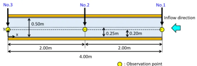
This examination is carried out by changing the observation variables, number and location of observation points. The computational conditions in this study is shown in Table 1. Com- putational model is shown in Figure 2.

Time increment  t , s 0.001

Time steps 2000

Number of nodes 153

Number of elements 200

Gravitational acceleration g , m/s

9.8

Lumping parameter e 0.8

Initial of estimated error covariance P

^1.0

Initial of estimated value ˆ



⁰

Convergence determination constant  0.01

Table 1: Computational conditions.

Figure 2: Computational model.

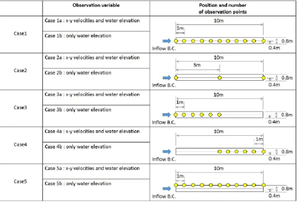
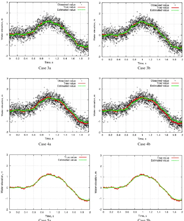
When the water elevation in amplitude 1.0m and period 2.0  s are given for the equation (5), the shallow water flow analysis is carried out. The results by this analysis are used as the artificial observation values. In this computation, the covariance for the system noise and ob- servation noise is set 0.0001 and 0.1, respectively. The system noise covariance matrix   Q and observation noise covariance matrix   ^R are the diagonal matrix that diagonal component are 0.0001 and 0.100. In addition, case ‘a’ represents that observation variables are flow ve- locity for x-y direction u , v and water  and case ‘b’ of setting that observation variable is  only. These cases are distinguished by subscript ‘a’ or ‘b’, number of observation points and position of observation points are shown in Figure 3. Experimental results are shown in Fig- ure 4 - 7.

Figure 3: Numerical test conditions.

In Cases 1-4, the observation points are set on center line of the channel, and number and

position of the observation points are changed. In Case 5, the observation points are set on

one side of the wall boundary.

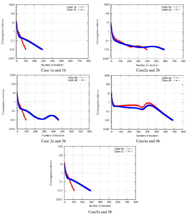
Case 1a and 1b Case2a and 2b

Case 3a and 3b Case4a and 4b

Case5a and 5b

Figure 4: Comparison of variation of convergence criterion.

Figure 4 shows comparison of variation of convergence criterion expressed by the Frobeni-

us norm. The equation of the Frobenius norm is shown in the flow chart of section 3.The con-

vergence criterion ε is set 0.01. This convergence criterion follows to the reference by

Heemink [3]. From this result, it was found that convergence rate in Case ‘a’ is faster than

that in Case “b” in the iterative computation of the predicted error covariance matrix.

Case 1a Case 1b

Case 2a Case 2b

Case 3a Case 3b

Case 4a Case 4b

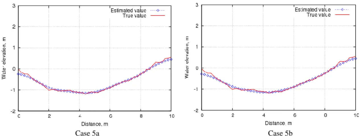
Case 5a Case 5b

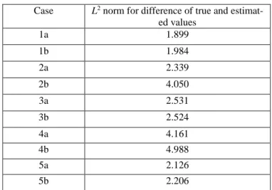
Figure 5: Comparison of distribution of estimated water elevation at T =2.0s.

Figure 6 shows the distribution of estimated water elevation of the channel center line at T =2.0s. In Case 1 and Case 2, estimated values are good agreement with the true value. In Case 3, when the observation points are set on the inflow boundary side, the estimated value is good agreement with the true value in the outflow boundary side region, but, In Case 4, when the observation points are set on the outflow boundary side, it was found that it is diffi- cult to estimate the distribution of the water elevation in inflow boundary side region. In Case 5, when the observation points are set on one side of the wall boundary, it was confirmed that the distribution of the water elevation is similar to that in Case 1.

Case 1a Case 1b

Case 2a Case 2b

Case 3a Case 3b

Case 4a Case 4b

Case 5a Case 5b

Figure 7: Comparison of time history of estimated water elevation at center point of channel ( x ^=5.0m, y =0.4m).

Figure 7 shows time history of estimated water elevation at center point of channel ( x =5.0m, y =0.4m). In all cases, observation noise is removed from observed value, and es- timated values are good agreement with the true value. Table 2 shows L

norm for difference of true and estimated values in Figure 7. In Case 3a and Case 3b, L

norm is approximately equivalent. In other cases, the value of L

norm in Case ‘a’ (the flow velocity for x and y di- rections and the water elevation are set as the observation variable) is less than that in Case

‘b’ (the water elevation is only set as the observation variable.). Therefore, it can be said that

estimated values in Case ‘a’ are better agreement with the true value than estimated values in

Case ‘b’.

Table 2: Comparison of L

norm for difference of true and estimated values.

5 CONCLUSIONS

In this study, flow field estimation analysis in open channel was carried out based on the Kalman filter FEM. The linear shallow water equation is employed as the governing equation, the Galarkin and the selective lumping methods are used to discretize the gov- erning equation in space and time, respectively. The conclusions in this study is shown as follows.

 It was seen that high accurate flow field estimation result is obtained in case that the ob- servation points are set to the downstream side in the open channel in comparison with the case that the observation points are set to the upstream side in the open channel.

 It was found that if the flow velocities for x and y directions and the water elevation are set as the observation variable in the computation of the flow field estimation, high accu- rate estimation result is obtained comparing to the case that the water elevation is only set as the observation variable.

APPENDIX

An example of flow field estimation using the practical measurement water elevation is shown in the appendix. The position of observation points and the size of the channel is shown in Figure 8, and the finite element mesh is shown in Figure 9. In addition, Table 3 shows the computational conditions in the flow field estimation. The flow field estima- tion analysis is carried out using the observed data at only points No.1 and No.2. The comparison of the time history of water elevation in case of the observed and the esti- mated values at points No.1 – No.3 is shown in Figures 10-12. From this result, it is found that though the flow field estimation can be carried out, there is difference between the observed and the estimated water elevation at point No.3. Therefore, it can be said that there is a possibility that flow distribution can’t be appropriately obtained, if a lot of observation points are not employed, and the period of the inflow wave is short. We sup- pose that this is one of the future work of this study.

Case

norm for difference of true and estimat- ed values

1a 1.899

1b 1.984

2a 2.339

2b 4.050

3a 2.531

3b 2.524

4a 4.161

4b 4.988

5a 2.126

5b 2.206

Figure 9: Finite element mesh.

Table 3: Computational conditions.

Total number of nodes

Total number of elements

Time increment  t , s

Number of time step

Lumping parameter e

Gravitational acceleration g , m/s

Water depth h , m

Driving matrix   

System error covariance matrix   ^Q

Observation error covariance matrix   ^R

Initial value of estimated error covariance matrix   P

Initial value of state vector   ˆ



Convergence criteria 

Figure 10: Comparison of water elevation at point No.1,

.

Figure 11: Comparison of water elevation at point No.2,

.

Figure 12: Comparison of water elevation at point No.3,

.

ACKOWDEDGEMENTS

This work was supported by Grants-in-Aid for scientific Research(C) Grant Number

15K05786.

ematical Modelling, Vol. 12(1988), pp.109-118.

[4] Toshimitsu Takagi, Kosuke Inamoto, Yutaka Hayakawa, Mutsuto Kawahara, Flow es-

timation of shallow water by the Kalman filter finite element method, Coastal engineer-

ing proceedings，Vol. 43，(1996), pp.346-350.