Shape optimization for stiffness maximization of geometrically nonlinear structure by considering fluid-structure-interaction

Paper No.21-00048

Shape optimization for stiffness maximization of geometrically

nonlinear structure by considering fluid-structure-interaction

Eiji KATAMINE

, Ryuga KAWAI

and Minori TAKAHASHI

∗_{Department of Mechanical Engineering, National Institute of Technology, Gifu College}

2236-2 Kamimakuwa, Motosu-shi, Gifu 501-0495, Japan E-mail: [email protected]

∗∗_{Deparment of Mechanical Engineering, Nagaoka University of Technology}

1603-1 Kamitomioka, Nagaoka-shi, Niigata 940-2188, Japan

Abstract

This paper presents numerical solution to a shape optimization for stationary fluid structure interactive fields. In the fluid structure interactive analysis, a weak coupled analysis is used to alternately analyze the governing equations of the flow field domain and the structural field considering geometrically nonlinear. A mean compliance minimization problem is formulated in order to achieve stiffness maximization on the structural field. Shape derivative, which means the sensitivity in the shape optimization problem, is derived theoretically by using the Lagrange multiplier method and adjoint variable method, and the formulae of the shape derivative with respect to domain variation of the distribution function. Reshaping is carried out by the H1_{gradient method proposed as an}

approach to solving shape optimization problems. Numerical analysis program for the problem is developed by using FreeFEM, and validity of proposed method is confirmed by numerical results of 2D problems.

Keywords : Shape optimization, Adjoint variable method, Finite element method, Fluid-structure-interactive, H1

gradient method

1. Introduction

Fluid-structure-interactive (FSI) problem is an interesting issue not only in mechanical engineering but also in fields such as marine engineering and bioengineering (Tsugawa and Takizawa, 2015). Moreover, in such an engineering field, the shape optimization problem for improving performance is an important issue, and in the bioengineering field, the problem of nonlinear structure is often dealt with. In this study, we discuss shape optimization of nonlinear structure for the FSI problem.

Shape optimization can be divided into topology shape optimization and shape optimization as one classification. Research on the shape optimization of FSI problem has been carried out by several researchers. Yoon (2010) proposed topology shape optimization using a monolithic formulation. Jenkins and Maute (2015) classified ”dry optimization”, which optimizes only the internal structure, and ”wet optimization”, which considers the shape of the fluid-structure interface as the design boundary, for the topology shape optimization of the FSI field, and then they analyzed the ”dry optimization” problem. Picelli et al. (2017) proposed an analysis method using an evolutionary topology optimization method. However, in these topology shape optimizations, linear strain was assumed in the structural field. For these, Lund et al. (2003), Jang et al. (2014), and Aghajari et. al. (2015) have performed analysis based on shape optimization assuming nonlinear strain on the structural field. In the studies on shape optimization conducted by Lund et al. (2003), Jang et al. (2014), and Aghajari et al. (2015), the design boundary was represented by a B-spline function and the design variables were minimized using a parametric analysis.

On the other hand, the authors have proposed solutions to fundamental shape optimization problems for maximizing the stiffness of the linear thermoelastic bodies (Katamine and Arai, 2017) and for minimizing the dissipative energy in viscous flow fields (Katamine et al. 2005), and demonstrated their validity. These solutions use the H1_{gradient method}

Ω

Ω

Γ

Γ

Γ

Γ

Γ

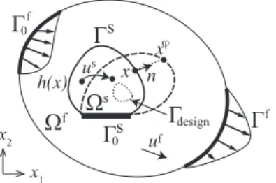
Fig. 1 Fluid–structure interaction problem. Viscous flow field domain,Ωf_{, has an inflow boundary,Γ}f

0, and an

outflow boundary,Γf_{. Elastic domainΩ}s_{has a known displacement boundary,Γ}s

0.

(Azegami, 1994, 2014). As the shape variations for shape optimization are expressed by domain variations of distribution systems in the H1 gradient method, nonparametric analysis can be performed without limiting the number of design variables that represent design boundaries.

This study considers to solve the shape optimization problem using the H1 _{gradient method for maximizing the}

stiffness of a structure by considering the geometric nonlinear strain in the stationary FSI. In the FSI analysis, a weak coupled analysis is used to alternately analyze the governing equations of the flow field domain and the structural field. Based on the above classification of Jenkins and Maute (2015), this study belongs to ”dry optimization” which optimizes the shape of only the internal structure. Shape derivative, which means the sensitivity in the shape optimization problem, is derived theoretically by using adjoint variable method, and the validity of proposed method is confirmed by numerical results of 2D problems.

2. FSI problem

Consider the stationary FSI field, as shown in Fig. 1. The viscous flow field domain,Ωf_{, has an inflow boundary,}

Γf

0, and an outflow boundary, Γ

f_{. In addition, elastic domain Ω}s _{has a known displacement boundary, Γ}s

0. Let the

common boundary between the fluid and elastic body beΓs_{. For simplicity, design boundaryΓ}

designfor shape optimization

represents the sub-boundary of elastic domainΩsand excludes boundaryΓs.

Owing to FSI, the elastic body at position x deforms with displacement us(x) and moves toward xφ = φ(x) (φ(x) =

xφ = x + us_{(x)). Further, let the unit normal vector at the boundary before deformation of the elastic body be n. In this}

study, the FSI analysis based on weak coupling is used.

2.1. Governing equations for elastic bodies

The governing equations based on the second Piola–Kirchhoff stress Σ(us(x)) is expressed as follows (Ciarlet, 1993):

−div((I + ∇us_(x))Σ(us_{(x)))= f}s_{(x), x ∈ Ω}s_{, (1)}

us(x)= 0, x ∈ Γs₀, (2)

(I+ ∇us(x))Σ(us(x))n= h(us(x)), x ∈ Γs, (3)

where fs(x) is the body force, h(us(x)) is the surface traction acting from the fluid side. Since the shape optimization problem shown later is formulated by only the state variables of the elastic body, the surface traction h is considered as a function of us_{(x). According to the Piola transformation (Ciarlet, 1993), h(u}s_{(x)) is expressed as follows:}

h(us(x))= T(x)n = (det∇φ(x)) Tφ(xφ) (∇φ(x))−Tn= (det(I + ∇us(x))) Tφ(xφ) (I+ ∇us(x))−T n, (4)

where T (x) denotes the stress tensor (the first Piola–Kirchhoff stress tensor) at the position prior to deformation x, and

Tφ(xφ) denotes one at the position after deformation xφ, which is called the Cauchy stress tensor. For simplicity, we will omit (x); for example, displacement us(x) as usin subsequent discussions.

The governing equation (1) above is multiplied by test functionws_(ws_{= 0 on Γ}s

0) and integrated over the domain. By

considering the symmetry of the second Piola–Kirchhoff stress, Σ(us_{), a weak formulation of the governing equation can}

be derived as follows:

as(us, us, ws)= ls(ws)+ ds(us, ws) ∀wsinΩs. (5) Note that terms as_(us_{, u}s_{, w}s_{), l}s_(ws_{), and d}s_(us_{, w}s_{) can be derived as follows:}

as(us, vs, ws)= ∫ ΩsΣ(ε s_(us_{)) : dε}s_(vs_)[ws_{] dx, l}s_(ws₎₌∫ Ωs f s_{· w}s_{dx, d}s_(us_{, w}s₎₌∫ Γsh(u s_{)· w}s_{dΓ, (6)}

whereεs(us) is Green–St Venant strain, defined as εs_(us₎₌ 1

2((∇u

s₎T_{+ ∇u}s_{+ (∇u}s₎T_(∇us_{)), (7)}

and the first variation dεs_(us_)[ws_{] is calculated as}

dεs(us)[ws]=1 2((∇w

s₎T_{+ ∇w}s₎₊1

2{(∇(u

s₎₎T_∇(ws_{)+ (∇(w}s₎₎T_∇(us_{)}. (8)}

StressΣ(εs_(us_{)) is expressed asΣ(ε}s_(us_{))= λ(trε}s_(us_{))I+ 2µ}s_εs_(us_{) with Lam´e constantsλ and µ}s_.

Given the surface traction, h, acting on the elastic body from the fluid side, elastic displacement us_{can be analyzed}

by applying the Newton–Raphson method to nonlinear term as(us, us, ws) of equation (5). The linearized weak form for given us_nat the n-th iteration and unknownδu_nsis represented as

das(u_ns, δus_n, ws)= as(us_n, u_ns, ws)− ls(ws)− ds(us, ws) ∀wsinΩs, (9) where, the first derivative, das_(us_{, v}s_{, w}s_{), for a}s_(us_{, v}s_{, w}s_{) is calculated as}

das(us, vs, ws)=

∫ Ωs{Σ(dε

s

(us)[vs]) : dεs(us)[ws]+ Σ(εs(us)) : d2εs(us)[vs, ws]} dx, (10) and the second derivative, d2εs(us)[δus, ws], forεs(us) is calculated as

d2εs(us)[δus, ws]=1 2((∇δu

s₎T_∇ws_{+ (∇w}s₎T_(∇δus_{)), (11)}

which is independent of us n.

2.2. Governing equations for flow fields

The weak forms of the Navier–Stokes and continuity equations with fluid densityρf and coefficient µf of viscosity in the flow field domain,Ωf, are given as (Katamine et al., 2005)

af(uf, wf)+ a₁f(uf, uf, wf)+ bf(p, wf)= 0 in Ωf, (12)

bf(q, uf)= 0 in Ωf. (13)

Note that terms af_(uf_{, w}f_{), a}f

1(u

f_{, u}f_{, w}f_{), and b}f_{(p, w}f_{) are defined as follows:}

af(uf, wf)= ∫ Ωf2µ f_εf_(uf_{) :ε}f_(wf_{) dx, a}f 1(u f_{, v}f_{, w}f₎₌∫ Ωfρ f_(uf_{· ∇v}f_{)· w}f _dx, bf(p, wf)= − ∫ Ωf ∇ · w f_{p dx, (14)} where uf _(uf _{is given onΓ}f

0) and p are the flow velocity and pressure, respectively, andw

f_(wf _{= 0 on Γ}f

0) and q are the

test functions. In addition, the stressσf_{(p, u}f_{) in flow field domain is defined as follows:}

σf_{(p, u}f_{)= −pI + 2µ}f_εf_(uf_{), ε}f_(uf₎₌1

2(∇u

f _{+ (∇u}f₎T_{). (15)}

2.3. Surface traction of elastic fields based on stress in the flow field domain

At the common boundary ofΓs_{on the deformed domain, the balance of the force is written as}

hφ(xφ)+ σf(p(xφ), uf(xφ))nf(xφ)= 0, where hφ(xφ) is surface traction after deformation xφ, (16)

with nf(xφ) = −nφ(xφ), which is the unit normal vector to the fluid domain at point xφ. According to the Piola trans-formation, surface tractions h(us_{(x)) and h}φ_(xφ_{) and unit normal vectors n and n}φ_{have the following relations (Ciarlet,}

1993):

h(us(x))= det∇φ(x)|∇φ(x)−Tn|hφ(xφ),

nφ= Cof∇φ(x)n

|Cof∇φ(x)n|, with Cof∇φ(x) = det∇φ(x)∇φ(x)−T. (17)

By combining these relations using|Cof∇φ(x)n| = det∇φ(x)|∇φ(x)−Tn|, h(us_{) is represented as}

h(us)= (det∇φ(x)) σf(p(xφ), uf(xφ)) (∇φ(x))−Tn= (det(I + ∇us))σf(p, uf) (I+ ∇us)−T n. (18)

The final elastic displacement us_{, flow velocity u}f_{, and pressure p in the FSI problem are then analyzed based on the}

2.4. Algorithm for FSI analysis

The analysis of FSI is performed by the following weak coupled scheme, and the common boundaryΓsand the fluid domainΩf _{are updated sequentially.}

Step 1.Define the common boundaryΓs_{between the fluid and elastic domain (iteration: k= 1, and u}s

k(x)= 0).

Step 2.For the deformed fluid domain Ω_kf(xφ), u_kf and pk are analyzed using equations (12) and (13), and the stress

σf

k(pk(xφ), u f

k(xφ)) at the common boundaryΓ s

kis calculated. If k< 2, the stress σ f k(pk(x), u f k(x)) at theΓ s kin the reference

fluid domainΩ_kf(x) is calculated.

Step 3.Calculate the hk(us_k(x)) using equation (18)．

Step 4.For the reference elastic domainΩs_{, u}s

k(x) is analyzed using equation (5).

Step 5.||us k(x)− u

s

k₋₁(x)|| is calculated, and if it is converged for iteration k, the analysis ends.

Step 6.Based on the us

k(x), the boundaryΓ s k(x) is moved toΓ s k+1(xφ= x + u s

k(x)), and the fluid domainΩ f

k(xφ) is updated

toΩ_kf₊₁(xφ) by k= k + 1, and returns to Step 2.

3. Shape optimization of structure in FSI field

This problem is formulated as follows:

Find Ωs_opt

that minimize ls(us)+ ds(us, us) (19)

subject to (5) and

∫

Ωsdx≤ M. (20)

Equation (19) is the objective functional indicating mean compliance considering the influence of the fluid field.∫_Ωsdx≤

M is the constraint equation in the structural domain, where M is the size of the initial domain. For simplification, we

ignore the domain variation of the boundaryΓs_{for the shape optimization.}

3.2. Shape derivative function

This problem can be formulated as a stationary problem without constraints by using the Lagrange multiplier method. In this case, the Lagrange function L(Ωs, us, ws, Λ) is given by the following equation:

L(Ωs, us, ws, Λ) = ls(us)+ ds(us, us) −as_(us_{, u}s_{, w}s_{)+ l}s_(ws_{)+ d}s_(us_{, w}s₎

+Λ(∫

Ωsdx− M), (21)

wherews_{is the adjoint variables for the governing equation in elastic domainΩ}s_{. Also,Λ is the Lagrange multiplier with}

respect to the domain size constraint.

Calculating for the shape derivative of L(Ωs, us, ws, Λ) with respect to domain variation for the elastic domain Ωs, the following conditional expressions can be derived with respect to the adjoint displacementws, and Lagrange multiplierΛ, based on optimality conditions for the shape optimization (Azegami, 1994, 2014):

∫ Ωs{Σ(dε s_(us_))[ws_{] : dε}s_(us_)[us′_{]+ Σ(ε}s_(us_{)) : d}2_εs_(us_)[ws_{, u}s′_{]} dx − d}s us(us, ws)[us′]− ls(us′) −ds′_(us_{, u}s_)[us′_{, u}s′_{]= 0 ∀u}s′_inΩs_{, (22)} Λ ≥ 0, ∫_Ωs dx≤ M, Λ( ∫ Ωs dx− M) = 0. (23)

Here, (· )′represents the derivative of the distribution function fixed in spatial coordinates with respect to the domain variation. In equation (22), the shape derivative ds′_(us_{, u}s_)[us′_{, u}s′_{] for d}s_(us_{, u}s_{) is represented as}

ds′(us, us)[us′, us′]= ∫ Γs{h ′_(us_)[us′_{]· u}s_{+ h(u}s_{)· u}s′_}dΓ =∫_Γs [

{(det(I + ∇us₎₎′_[us′_]σf_{(p, u}f_{) (I+ ∇u}s₎−T _{n+ (det(I + ∇u}s_))σf_{(p, u}f_{) ((I+ ∇u}s₎−T₎′_[us′_{] n} · u}s

+h(us_{)· u}s′]_dΓ

=∫_Γs [

{∇ · us′_σf_{(p, u}f_{) (I+ ∇u}s₎−T _{n− (det(I + ∇u}s_))σf_{(p, u}f_)∇us′_{n} · u}s_{+ h(u}s_{)· u}s′]_{dΓ. (24)}

To obtain (24), we used the shape derivatives for domain Jacobi determinant and domain Jacobi inverse matrix (Azegami, 2020, section 9.2.1), which is (det(I+ ∇us₎₎′_[us′_{]= ∇ · u}s′_{and ((I+ ∇u}s₎−T₎′_[us′_{]= −∇u}s′_{. Also, the shape derivative}

ds_us(us, ws)[us′] for ds(us, ws) in (22), where (· )us= ∂( · )/∂us, is represented as d_uss(us, ws)[us′]=

∫

The shape derivative function ¯g = gsn, which shows the sensitivity on the design boundaries for the shape

optimiza-tion, can be derived as follows: gs_{= −Σ(ε}s

(us)) : dεs(us)[ws]+ fs· (us+ ws)+ Λ. (25)

As the shape derivative function ¯g can be derived for this problem, the H1_{gradient method, called the traction method}

assuming linear strain for the domain variation of elastic domain (Azegami, 2014, section 9.2), can be applied for this shape optimization problem.

Calculation of shape derivative function Domain variation analysis by H gradient method Updating shape with domain variation for elastic domain

Convergence? Yes No Final design Initial design FEM FEM

Flow field analysis u = u + u_(n)

(n+1) f f f

Elastic field analysisu = u + u(n+1) (n) s s s

Objective Functional FSI problem

Convergence?

Adjoint elastic field analysis FEM

Weak coupling analysis

(n)

(n)

1

δ δ

Fig. 2 Numerical analysis procedure for shape optimization

x₁ x₂

Γ

Γ

Γ

Ω

Γ

Ω

w

L

L

Fig. 3 For the structure on the cavity flow,

the stiffness maximization problem is set with the circular holes as the design boundaries.

3.3. Numerical Analysis procedure for shape optimization

The proposed shape optimization analysis can be performed by repeating the following steps (shown as Fig. 2): Step 1.Give initial shape.

Step 2.Analyze the elastic displacement, us, flow velocity uf, and pressure p in the FSI problem by using the weak coupling analysis based on the algorithm of section 2.4.

Step 3.Stop when the objective functional has converged.

Step 4.Analyze the adjoint elastic displacement,ws_{, based on the adjoint equation (22).}

Step 5.Calculate the shape derivative function, ¯g, based on the equation (25).

Step 6.Analyze the domain variation based on the H1gradient method to update the elastic domain. Return to Step 2.

4. Numerical examples

In this study, the numerical analysis program was developed using FreeFEM (Ootsuka and Takaishi, 2014). Based on Algorithm 1b in the tutorial (Suzuki, 2018), the FSI field was analyzed using the P2/P1 elements for the flow velocity and pressure of the flow field and the P2 element for the displacement of the elastic field. Moreover, for analyzing the FSI, the fixedborder option of FreeFEM was used to prevent reassignment of the finite element nodes at the common boundary, Γs_{, of elastic domainΩ}s_{and flow field domainΩ}f_.

p 2000 0 -2000 -4000 -6000 -8000 -10000 -12000 -14000 -16000 -18000 -20000 -22000 -24000 -26000 -28000 p 2000 0 -2000 -4000 -6000 -8000 -10000 -12000 -14000 -16000 -18000 -20000 -22000 -24000 -26000 -28000

Flow velocity Pressure distribution Flow velocity Pressure distribution

(a) E= 6 kPa (Linear) (b) E= 6 kPa (Non-linear)

Fig. 4 Flow velocity and pressure distribution for flow field on cavity flow, there is almost no difference in the flow field, as compared with the comparison of linear and non-linear in the initial shape.

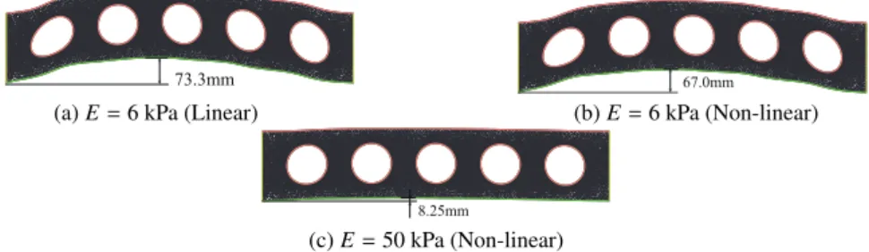
73.3mm 67.0mm (a) E= 6 kPa (Linear) (b) E= 6 kPa (Non-linear)

8.25mm

(c) E= 50 kPa (Non-linear)

Fig. 5 Deformed shape (Initial) for structure on cavity flow. Comparing (a) E= 6 kPa (Linear) and E = 6 kPa (Non-linear), the deformation of Case (b) is smaller due to the effect of the lifting effect based on the geometrically nonlinear.

55.1mm 53.6mm

(a) E= 6 kPa (Linear) (b) E= 6 kPa (Non-linear)

6.23mm

(c) E= 50 kPa (Non-linear)

Fig. 6 Deformed shape (Optimized) for structure on cavity flow. For all cases, the amount of deformation is smaller than the initial shape of Fig. 5, and the stiffness is improved.

4.1. Structure on cavity flow

We analyzed the structure on the cavity flow, as shown in Fig. 3. For the boundary conditions in the viscous flow field, a flow velocity was applied on the left boundary and set to zero at the other boundaries. For the boundary conditions in the structure, the left and right boundaries were fixed, while the lower boundary was set asΓsbetween the fluid and structure. With a flow velocity on the left side of uf = 1 m/s, density ρf and coefficient of viscosity µf were set such that the Reynolds number was Re = 100. In addition, Poisson’s ratio was set as ν = 0.3, and Young’s modulus was set as

E = 6 kPa or E = 50 kPa. For E = 6 kPa, we performed an analysis by assuming linear strain. Then, Lam´e constants λ

andµs_{were calculated based on Young’s modulus E and Poisson’s ratioν as λ =} E_ν

(1+ν)(1−2ν) andµ

s₌ E

2(1+ν), respectively.

For the model dimensions, L= 1 m and w = L/5 m. The holes in the structure were set as the design boundaries, Γs design,

and body force fswas disregarded.

Figures 4 to 7 show the numerical results. Figure 4 shows the flow velocity and pressure distributions for the deformed flow field for the initial shape of the cases of E = 6 kPa (Linear) and E = 6 kPa (Non-linear). Based on Fig.4 and Fig.5, it can be confirmed that there is a difference in the deformation of the structure, but the difference in the flow field is slightly, as compared with the comparison of linear and non-linear in the initial shape. As shown in Fig. 5(c), when E= 50 kPa, the deformation was so small that nonlinearity could be ignored. The comparison of Figs. 5 (a) and (b) shows that when E= 6 kPa, the amount of deformation is smaller in Fig. 5 (b), where nonlinearity is considered. This is because of the deformation restraining phenomenon called the lifting effect (Izui and Sakai, 2010), which is characteristic of the geometrically nonlinear structure of the beams fixed at both ends. Figures 6 shows the deformed state for optimized shapes. The optimized shapes shown in Figs. 7 (a) and (c) are similar because in Fig. 7 (c), the Young’s modulus is large

(a) E= 6 kPa (Linear) (b) E= 6 kPa (Non-linear)

(c) E= 50 kPa (Non-linear)

Fig. 7 Initial and optimized shapes (Dashed line: Initial, Solid line: Optimized) for structure on cavity flow. In Case (c), Young’s modulus is large and nonlinearity is not appeared, so the optimum shapes of Case (a) and (c) are similar. The comparison between Cases (a) and (b) shows the results for consideration of geometrically nonlinear.

Γf 0 Γ f Γ₀s Γs Γdesign Ωf Ωs L D h w x1 x2 s

Fig. 8 For the obstacle in channel, the stiffness maximization problem is set with the circular holes as the design boundaries. p 6 5 4 3 2 1 0 -1 -2 -3 -4 -5 -6 -7 -8

(a) Flow velocity distribution (b) Pressure distribtion

Fig. 9 Flow velocity and pressure distribution for flow field on obstacle problem in channel, Case of E= 5 kPa (Non-linear)

enough that the effect of nonlinearity is not observed. In contrast, the comparison of Figs. 7 (a) and (b) shows that the effect of nonlinearity appears in the optimized shape in Fig. 7 (b). In addition, the objective functional decreased by 26% for E = 6 kPa(linear), 23% for E = 6 kPa(nonlinear), and 26% for E = 50 kPa(nonlinear), and the stiffness improved with constant domain size. In Fig. 6, the stress concentration part can be seen. However, since the purpose of this study is to maximize the stiffness, not the strength, it is unavoidable. In fact, the similar results can be seen in other studies (Azegami, 2020, Katamine and Arai, 2017) on shape optimization for stiffness maximization based on minimizing mean compliance.

4.2. Obstacle in pipe channel flow

The problem is shown in Fig. 8. For the boundary conditions in the flow field, a Poiseuille flow was applied to the left boundary, the right boundary was set as a natural boundary, and the flow velocities at the upper and lower boundaries were set to zero. For the boundary conditions in the structure, the lower boundary was fixed and the other boundaries were set as the common boundaries,Γs, between the fluid and structure. With a maximum flow velocity on the left side of uf = 1 m/s, density ρf and coefficient of viscosity µf were set such that the Reynolds number was Re= 100. We set Poisson’s ratioν = 0.3 and Young’s modulus as E = 5 kPa (nonlinear) and E = 40 kPa (nonlinear). The model dimensions were set as D= 4 m, L = 16 m, h = D/4 m, w = h/5 m, and the distance from the inflow boundary, Γ₀f, to the center of the obstacle was L/4 m. The boundaries with initially round shapes inside the obstacle were set as Γs

desi_gn, and body force

fs_{was disregarded.}

Figures 9 to 10 show the numerical results. Figure 9 shows the flow velocity and pressure distributions for the

231mm 212mm 35.2mm 31.9mm

(a) E= 5 kPa (b) E= 40 kPa

Fig. 10 Deformed shapes (Initial and optimized) and initial and optimized shapes (Dashed line: Initial, Solid line: Optimized) for obstacle in channel. The optimum shapes of Case (b) are almost symmetric with respect to the left and right side of the obstacle, with a negligible effect of nonlinearity. In contrast, Case (a), the effect of nonlinearity was large, and thus the optimum shapes lost symmetry.

deformed flow field for the case of E= 5 kPa. Figure 10 shows the numerical results, with a large deformation in Fig. 10 (a) E= 5 kPa such that the deflection exceeds the obstacle width. In contrast, the deformation in Fig. 10 (b) E = 40 kPa is very small. For the optimized shapes in Fig. 10 (b), the shapes are almost symmetric with respect to the left and right side of the obstacle, with a negligible effect of nonlinearity. In contrast, in Fig. 10 (a), the effect of nonlinearity was large, and thus the shapes lost symmetry. The objective functional decreased by 13% for E = 5 kPa and 15% for E = 40 kPa, this showing an improvement in the stiffness.

5. Conclusions

In this paper, we discussed a shape optimization problem for maximizing stiffness of a geometrically nonlinear structure by considering stationary FSI. We formulated the problem, derived the shape derivative function for the problem, and presented examples of numerical analysis using the H1_{gradient method to show the validity of the proposed solution.}

Acknowledgments

The advice on FSI problem of Dr. Atsushi Suzuki, Osaka University in Japan, was helpful in conducting the present study. The present study was supported in part by The OGAWA Science and Technology Foundation in Japan.

References

Aghajari, N. and Schafer, M., Efficient shape optimization for fluid-structure interaction problems, Journal of Fluids and Structures, Vol. 57, (2015), pp.298–313.

Azegami, H., Solution to domain optimization problems (in Japanese), Transactions of the Japan Society of Mechanical Engineers, Series A, Vol. 60, (1994), pp.1479–1486. (in Japanese)

Azegami, H., Regularized solution to domain optimization problems, Transactions of the Japan Society for Industrial and Applied Mathematics, Vol.24, No.2, (2014), pp.83–138.(in Japanese)

Azegami, H., Shape optimization problems (2020), Springer.

Ciarlet, P. G., Mathematical Elasticity, Volume 1: Three Dimensional Elasticity (1993), Elsevier.

Izumi, S and Sakai, S., Practical finite element method simulation (2010), pp. 69–70, Morikita, Tokyo. (in Japanese) Jang, H. L. and Cho, S., Adjoint shape design sensitivity analysis of fluid-solid interactions using concurrent mesh velocity

in ALE formulation, Finite Elements in Analysis and Design, Vol.80, (2014), pp.20-32.

Jenkins, N. and Maute K., Level set topology optimization of stationary fluid-structure interaction problems, Structural and Multidisciplinary Optimization, Vol.52, (2015), pp.179–195.

Katamine, E. and Arai Y. , Multi-objective shape optimization for maximizing stiffness in thermo-elastic fields, Trans-action of the Japan Society of Mechanical Engineers, Vol.83, No. 845, (2017), DOI:10.1299/transjsme.16-00490, 13pages. (in Japanese)

Katamine, E., Azegami, H., Tsubata, T. and Ito, S., Solution to shape optimization problems of viscous flow fields, International Journal of Computational Fluid Dynamics, Vol. No.1, (2005), pp.45–51.

Lund, E., Moller, H. and Jakobson, L. A., Shape design optimization of stationary fluid-structure interaction problems with large displacements and turbulence, Structural and Multidisciplinary Optimization, Vol.25, (2003), pp.383–392. Ootsuka K. and Takaishi, T., Finite element analysis using mathematical programming language FreeFem++, Kyoritsu,

2014. (in Japanese)

Picelli, R., Vicente W. M. and Pavanello, R., Evolutionary topology optimization for structural compliance minimization considering design-dependent FSI loads, Finite Elements in Analysis and Design, Vol.135, (2017), pp.44-55. Suzuki, A., FreeFem++ tutorial: Fluid-structure interaction problem –balance of the surface force and domain

defor-mation in a weak coupling method– (online), available from [https: //www.ljll.math.upmc.fr/-suzukia/FreeFempp-tutorial-JSIAM2018/PDF/tutorial-JSIAM2018.pdf], (accessed on Nov. 21, 2020).

Tsugawa, Y. and Takizawa, K., Computational fluid-structure interaction methods and applications (2015), Morikita. (in Japanese)

Yoon, G. H., Topology optimization for stationary fluid-structure interaction problems using a new monolithic formula-tion, International Journal for Numerical Method in Engineering, Vol.82, (2010), pp.591-616.