固液界面ナノバブルと吸着気体分子層に関する実験 的研究

九州大学学術情報リポジトリ

Kyushu University Institutional Repository

固液界面ナノバブルと吸着気体分子層に関する実験 的研究

手嶋, 秀彰

http://hdl.handle.net/2324/4060171

出版情報：九州大学, 2019, 博士（工学）, 課程博士 バージョン：

権利関係：

固液界面ナノバブルと吸着気体分子層 に関する実験的研究

博士 ( 工学 ) 学位論文

九州大学大学院 工学府航空宇宙工学専攻

手嶋 秀彰

令和元年１２月

I

第 1 章 序章 ... 1

1.1. はじめに ... 1

1.2. 界面ナノバブル ... 2

1.2.1. 特性 ... 3

1.2.1.1 接触角 ... 3

1.2.1.2 長寿命 ... 6

1.2.1.3 外乱に対する超安定性 ... 7

1.2.2. 生成方法 ... 11

1.2.2.1 溶媒交換法 ... 11

1.2.2.2 マイクロ波照射 ... 12

1.2.2.3 電気分解 ... 13

1.2.3. 理論 ... 14

1.2.3.1 コンタミネーション理論 ... 14

1.2.3.2 動的平衡理論 ... 15

1.2.3.3 ピニングとガス過飽和 ... 17

1.2.4. より厚みが薄い吸着気体分子層 ... 19

1.2.4.1 マイクロパンケーキ ... 21

1.2.4.2 整列層と非整列層 ... 21

1.3. イメージング ... 23

1.3.1. 光学顕微鏡 ... 23

1.3.2. 透過型電子顕微鏡 ... 24

1.3.3. 原子間力顕微鏡 ... 25

1.3.3.1 振幅変調(Amplitude modulation: AM)モード ... 27

1.3.3.2 ピークフォースタッピング(Peakforce tapping: PFT)モード ... 27

1.3.3.3 周波数変調(Frequency modulation: FM)モード ... 29

1.4. 研究目的 ... 30

1.5. 論文の構成 ... 30

第2章 探針の濡れ性がナノバブル計測に与える影響 ... 31

2.1. 概要 ... 31

2.2. 探針の作製 ... 31

2.3. 試料と計測の準備 ... 33

2.4. PFTモードによる界面ナノバブル観察 ... 34

2.5. 界面ナノバブル形状の再構築... 39

2.6. まとめ ... 43

第3章 界面ナノバブルのピニング ... 44

II

3.1. 概要 ... 44

3.2. 三相界線に働く力 ... 44

3.2.1. 線張力 ... 44

3.2.2. ピニング ... 46

3.3. 界面ナノバブルのピニングの定量的な評価... 47

3.4. 三相界線の縮小と拡大 ... 51

3.5. 合体した界面ナノバブルの安定性 ... 54

3.6. 界面ナノバブルの生成メカニズム ... 57

3.7. まとめ ... 59

第4章 吸着気体分子層と水和構造 ... 60

4.1. 概要 ... 60

4.2. 試料と計測の準備 ... 60

4.3. 吸着気体分子層の可動性 ... 61

4.4. 水和構造の計測 ... 69

4.4.1. 水和構造 ... 69

4.4.2. 高さ像と周波数シフトカーブの比較... 70

4.4.3. 気体分子が水和構造に与える影響 ... 78

4.4.4. 吸着気体分子層がある場合と無い場合の水和構造... 79

4.5. まとめ ... 81

第5章 総括 ... 82

参考文献 ... 84

謝辞 ... 94

付録 ... 96

付録1 コンタミネーションの混入 ... 96

付録2 FMモード計測中の探針の押し込み強さ ... 101

付録3 FMモード計測中の熱ドリフトの影響... 102

付録4 探針のダメージがFM計測に与える影響 ... 104

付録5 加熱に対する界面ナノバブルの超安定性の理論的検討 ... 106

III

Lists of Figures

Figure 1.1 Three-dimensional image of interfacial nanobubbles obtained by AFM. ... 2 Figure 1.2 A photo of an HOPG and a schematic image of step and terrace structures on an HOPG surface. ... 5 Figure 1.3 Stability of nanobubbles with time at different ambient temperature, where the temperature of liquid is 30 °C: (A) 20 min at 21 °C, (B) 2 days at 21 °C, (C) an additional day at 23 °C, (D) a second additional day at 25 °C (the start of day 5). Some small bubbles dissolved on the third day[9]. ... 7 Figure 1.4 Cavitation activity (left), and corresponding nanobubble density (right) imaged by AFM (topography images) for various probes. The length scales given in (A) also refer to (B), (C), and (D). (A) and (B): polyamide substrates; (B) after ethanol-water exchange. (C) and (D): hydrophobized silicon substrates; (D) after ethanol-water exchange. There is hardly any cavitation though the substrates are densely covered by surface nanobubbles.

Note that the cavitation bubbles in (A) emerge exclusively from microscopic cracks in the surface, whereas the whole substrate is covered by nanobubbles. The cavitation bubbles in (C) presumably originate from surface contaminations[53]. ... 8 Figure 1.5 (a) Schematic representation of the modified closed fluid cell for in situ ultrasound application and tapping-mode AFM imaging; (b) the crosssectional profiles of three pairs of nanobubbles. Tapping mode AFM height images of nanobubbles are shown in (c) prior to sonication and (d) after sonication for 40 s. The scale bars for (c) and (d) are identical and the scan size is 5 × 5 m²[54]. ... 9 Figure 1.6 Microbubbles nucleated on highly oriented pyrolytic graphite (HOPG) at elevated temperature. (a) Microbubbles formed on HOPG directly exposed to water at 85 °C. (b) After solvent exchange, no microbubbles formed on HOPG at 95 °C. (c) Microbubbles formed again when HOPG was dried after the solvent-exchange process and exposed to water at 85 °C. (d−f) AFM images of HOPG under the same conditions as in a−c, now at room temperature. The area of the AFM images is 5 μm × 5 μm[56]... 10 Figure 1.7 (a) Optical image of nanobubbles in the water phase at 90 °C and (b) the corresponding image of the very same location after the three-phase contact line has passed with microdroplets in the gas phase, with the entrapped nanobubbles. In (b), the temperature is 95 °C. The nanobubbles and resulting droplets are marked with various colors to assist recognition. The patterns of the marks on the surface in (a) are identical to those in (b), demonstrating that all nanobubbles nucleate microdroplets. Also shown are some spontaneously nucleated microdroplets[29]. ... 10 Figure 1.8 (a) Schematic diagram of nanobubble generation via microwave. Effect of (b) microwave

IV

irradiation time, (c) microwave power, and (d)dissolved oxygen concentration on the formation of nanobubbles[66]. ... 13 Figure 1.9 (a) Schematic picture of dynamic equilibrium theory. (b) Gas outflux 𝑗out and influx 𝑗in into the surface nanobubble as function of bubble radius R. The crossing point defines the equilibrium footprint radius L. The units of 𝑗 are m3/s. If the slope of 𝑗out at L = 0 is larger than that of 𝑗in , no surface nanobubbles can emerge. The detailed data to illustrate this plot is written in [84]. ... 16 Figure 1.10 (a) Sketch of the shrinking process of a pinned surface nanobubbles with initial contact angle 𝜃𝑖: Due to the pinning, footprint is fixed. Shrinking thus implies a decrease in 𝜃 and height and an increase in the radius of curvature. Therefore, the Laplace pressure inside the bubble reduces and eventually becomes too weak to further press out the bubble against the oversaturation. (b) Equilibrium contact angle 𝜃𝑒 of a nitrogen bubble in water as function of the lateral footprint diameter L for four different oversaturations 𝜁 = 0.25, 0.5, 1.0, 2.0, bottom to top[88]. ... 19 Figure 1.11 Micropancakes and nanobubble-pancake composites formed after solvent exchange method: (a) height image, (b) section of the height image, and (c) phase image of micropancakes; (d) height image, (e) section of the height image, and (f) phase image of nanobubble-pancake composites[38]. ... 20 Figure 1.12 Change of micropancakes and nanobubbles as a function of time and temperature: (a) initial pancakes (P = micropancake) immediately after the displacement of ethanol with water at 31 ± 0.5 °C; (b) after 1.5 h at 31 ± 0.5 °C, P1 and P2 coalesced into a bigger micropancake, P3 (the nanobubbles on the micropancakes could move with time, for example, the one inside the dotted circle); (c) after another 1.5 h at this temperature, the pancakes are not very different from those in image b; (d) recommencement of growth of P3 if the temperature is increased to 36 ± 0.5 °C and held for 0.5 h[38]. ... 20 Figure 1.13 FM-AFM image of an HOPG surface in water after exposure to nitrogen for 160 min.

Three arrows indicate the three row orientations[18]. ... 22 Figure 1.14 Simultaneous microscopy of nanobubbles. (a) Bubbles are nucleated by solvent exchange within a removable channel. (b) TIRF image of the bubbles. (c) AFM image of the same feature. A bright spot in the middle (white arrow) corresponds to the location of the AFM tip. The scale bars in (b) and (c) are 5 μm[46]. ... 24 Figure 1.15 Time evolution of different kinds of double nanobubbles. (a, b) The snap shots of TEM images showing the merging of adjacent two nanobubbles observed for 15 and 50 seconds, respectively. When the nanobubble sizes are significantly different, it shows an Ostwald ripening-like merging process, whereas the similar-sized bubbles are coalescing as their inter-bubble boundary breaks. Scale bars are 10 nm... 25

V

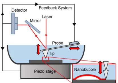
Figure 1.16 (a) Schematic image of interfacial nanobubble observation by using AFM. ... 26 Figure 1.17 (a) Cross-sectional data points (circles) along the scanning direction of a nanobubble observed in [99]. (b) Same bubble showing raw and deconvoluted cross-sectional data points (blue and red circles, respectively) together with their respective spherical fits Rc’ and Rc. Alternatively, Rc can be obtained using the tip radius Rt through Rc= Rc’- Rt[99].

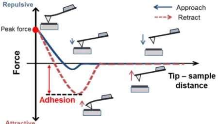
... 26 Figure 1.18 Measurement of a force curve between a solid surface and an AFM tip. Blue and red curves indicate the force curves in the approach and retraction, respectively. Adhesion force corresponds to the maximum value of the attractive force in the retraction period, allowing one to sensitively visualize the existence of nanoscale gas phases. ... 28 Figure 1.19 AFM height images of PDMS nanodroplets and a nanobubble in PeakForce mode. (a−e) Successive AFM images captured for peak forces Fp = 0.5, 1.0, 3.0, 5.0, and 10.0 nN. A final scan was taken at Fp = 0.5 nN, showing that the objects were not destroyed by the scanning. Scan size: 2 m × 1 m. Height scale: (a−d, f) 50 nm and (e) 5 nm[106]. ... 29 Figure 1.20 Schematic image of measurement of a hydration structure using FM-AFM. ... 30 Figure 2.1 SEM images of an AFM tip (a) before and (b) after Teflon coating, i.e., the unprocessed tip and the hydrophobic tip. Scale bars are 5 m. ... 32 Figure 2.2 AFM images (5 × 5 m) of the interfacial nanobubbles scanned using (a, b) hydrophobic, (c, d) unprocessed, and (e, f) hydrophilic tips. The height images (a), (c), and (e) and adhesion images (b), (d), and (f) were acquired at the same time, respectively. The peak force setpoint was constant at 300 pN in all experiments. The scale bar is 1 m. The red circles indicate the nanobubbles on which the force curves were measured. The green circles indicate the nanobubbles which can be seen in the adhesion images only. ... 34 Figure 2.3 Force curves between interfacial nanobubbles and (a) hydrophobic, (b) unprocessed, and (c) hydrophilic AFM tips. The blue curve and red curve indicate the force curves in the approach and retraction, respectively. The interactions between the nanobubbles and the tips are drawn in the insets. The hydrophobic and unprocessed tips penetrate the gas/liquid interface and experience repulsive and attractive forces owing to the pinning of the three- phase contact line at the tip surfaces. In contrast, the hydrophilic tip does not penetrate the interface and experiences the forces through the thin liquid film between the tip and the nanobubbles. ... 36 Figure 2.4 Height images of nanobubble-like objects obtained by a hydrophilic AFM tip.

Measurements were performed with peak force setpoints of 0.3, 1.0, and 5.0 nN in the same area. Scale bar is 1 m. ... 38 Figure 2.5 Schematic diagram of the underestimation of the nanobubble profile. The pinning position at the surface of the tips determines the degree of underestimation. ... 39

VI

Figure 2.6 (a) Penetration depth 𝛿 [calculated from Eq. (4)] scanned with the hydrophobic, unprocessed, and hydrophilic tips, and plotted as a function of 𝑟true; (b) scatter plot of ℎtrue [calculated from Eq. (1)] versus ℎapp ; (c) 𝑟true plotted versus 𝑟app . The broken lines shown in (b) have a slope of 1.0. Linear regressions obtained by least-squares fitting are shown by the solid lines in (c). Since the true height cannot be estimated from nanobubbles whose apparent footprint radius is zero, they are not plotted in (b). The plots with zero apparent footprint radius value are not included in the linear regression estimations in (c). ... 41 Figure 3.1 Schematic drawing of line tension working on a three-phase contact line of a surface bubble.

This tension is attributed to the imbalance of intermolecular force along the contact line and thus depends on the curvature of footprint radius. ... 46 Figure 3.2 Schematic diagram of the surface tension and pinning force working at three-phase contact line of an interfacial nanobubble. ... 47 Figure 3.3 Topographical PF-QNM images (5 × 5 μm) of HOPG/water interfacial nanobubbles. The images were obtained at (a) 45 min, (b) 90 min, (c) 150 min, (d) 150 min (adhesion image), (e) 180 min, and (f) 230 min after solvent exchange with a setpoint of 903 pN, 770 pN, 2.62 nN, 2.62 nN, 462 pN, and 462 pN, respectively. The white circles, marked as (1), (2), and (3) indicate shrinking nanobubbles. The blue circles marked as (4), (5), and (6) indicate the bubbles whose footprint radius increased. The white lines in (f) indicate the positions of the steps on the HOPG surface. The broken lines marked as (i), (ii), and (iii) indicate the spherical and neck regions of a coalesced nanobuble. ... 48 Figure 3.4 Scatter plot of the pinning force as a function of footprint radius. The pinning forces were calculated from Equation (3.3). ... 50 Figure 3.5 Change of the shape of small and large interfacial nanobubbles due to scanning with strong load forces. The deformed shape is kept due to strong pinning force. Some scale is not correct for clarity. ... 51 Figure 3.6 Behavior of (a, c, e, and g) small and (b, d, f, and h) large nanobubbles flattened by strong load force scanning. ... 54 Figure 3.7 Cross sections of the coalesced nanobubble marked by the white square in Figure 3.3(b).

Cross sections (i) and (ii) show the semispherical parts, and (iii) shows the joint part. . 55 Figure 3.8 Coalesced nanobubbles marked by the white square in Figure 3.3(b). The metastability of coalesced nanobubbles results from strong pinning forces on the semispherical parts... 56 Figure 3.9 Mechanism of nanobubble nucleation during solvent exchange method. (a) Several layers of gas molecules are formed through solvent exchange. (b) Small nanobubbles have a high pinning force, which prevents dissolution owing to the higher Laplace pressure. (c) Large nanobubbles have a lower pinning force and additional gas can diffuse into the

VII

bubbles because of the lower Laplace pressure. ... 58 Figure 4.1 (a, b) Height images (2 m × 2 m) of the HOPG/pure water interface obtained with cantilever peak-to-peak oscillation amplitudes of approximately 4 and 0.8 nm, respectively. The red arrows indicate micropancakes, and the blue arrows indicate disordered gas layers. (c) Higher resolution height image (200 nm × 200 nm) of nanoscopic gas phases. The yellow arrows indicate the direction of ordered gas molecules.

The height profile measured along the white dot lines (1, 2) are shown in Figure 4.2. .. 62 Figure 4.2 Height profiles of interfacial gas phases observed in Figure 4.1(b, c). Cross sections (1-2) are corresponding to the white dot lines (1-2) in Figure 4.1(b, c). Red arrow indicates the profile of a micropancake. Blue and yellow arrows indicate the profiles of disordered and ordered gas layers, respectively... 63 Figure 4.3 Change of interaction time between an AFM tip and a sample surface with respect to oscillation amplitudes of the AFM tip. ... 64 Figure 4.4 Magnified images of a micropancake on a disordered gas layer in the area surrounded by a white broken line in Figure 4.1(b). The image (a) was composed of the scanning data from left side to right side (i.e., a trace image) and (b) was obtained by scanning in the opposite direction (i.e., a retrace image). The red line indicates the shape of the micropancake. The black broken line indicates the edge of the disordered gas layer. ... 65 Figure 4.5 Proposed mechanism for the generation of ordered and disordered gas layers and mobile micropancakes. (a) Adsorption of dissolved gas molecules on the HOPG surface.

Dissolved and adsorbed gas molecules are indicated by white and gray circles, respectively. (b) Nucleation of micropancakes on solidlike disordered gas layers covering ordered gas layers. (c) Pinning of mobile micropancakes at the boundary between the disordered gas layers and ordered gas layers. Some structures are not represented to scale for clarity. ... 66 Figure 4.6 Height images (5 × 5 m) of the HOPG/pure water interface (a, b) before and (c) after adding degassed water. Panels (a) and (b) show the trace and retrace images, respectively.

The green circles indicate that mobile micropancakes disappeared in image (c). The broken white lines shown in (a) and (c) are corresponding to (d) the red and blue cross sections, respectively. ... 68 Figure 4.7 Analysis of the bare HOPG/pure water interface. (a) Height image (3 µm × 3 µm). Scale bar is 500 nm. (b) 2D frequency-shift map during approach. Scale bars represent 5 nm (horizontally) and 3 nm (vertically). (c) Averaged frequency shift–distance curves at the interface. The red and blue curves indicate the frequency-shift curves during approach and retraction, respectively. The peak-to-peak oscillation amplitude of the AFM tip is approximately 0.8 nm. The preset frequency shifts are +83 and +666 Hz in (a) and (b,c),

VIII

respectively. ... 71 Figure 4.8 HOPG surface with adsorbed gas layers. (a) Height image (2 µm × 2 µm). Scale bar is 500 nm. (b) Magnified image (0.5 µm × 0.5 µm) in the area surrounded by the white broken line in (a). Scale bar is 100 nm. (c) 2D frequency-shift map in the approach. Scale bars represent 5 nm (horizontally) and 2 nm (vertically). (d) Averaged frequency shift curves on the adsorbed gas layers. The red and blue curves indicate the frequency curves in the approach and retraction. The peak-to-peak oscillation amplitude of the AFM tip was 0.8 nm. The preset frequency shift was +83 Hz. ... 73 Figure 4.9 HOPG surface with adsorbed gas layers under high load force. (a) Height image (2 µm × 2 µm). Scale bar is 500 nm. (b) 2D frequency-shift map in the approach. Scale bars represent 5 nm (horizontally) and 2 nm (vertically). (c) Averaged frequency shift–distance curves when penetrating the adsorbed gas layers. The red and blue curves indicate the frequency-shift curves in the approach and retraction, respectively. The peak-to-peak oscillation amplitude of the AFM tip was approximately 4.0 nm in (a) and 0.8 nm in (b, c). The preset frequency shifts were +83 Hz in (a) and +666 Hz in (b, c). ... 75 Figure 4.10 Frequency shift curves on a bare HOPG surface and inside adsorbed gas layers. The black arrows indicate the regions where the molecular density of water is high (hydration layers).

The green arrows indicate the regions where the molecular density of gas is high (each gas layer) in the approach curve. The data are from Figure 4.7(c) and Figure 4.9(c). .... 76 Figure 4.11 Analysis of the HOPG/pure water interface with nanoscopic gas phases obtained with the hydrophobic AFM tip. (a) Height image (3 µm × 3 µm). (b, c) 2D frequency-shift maps in the approach and retraction, respectively. (d) Averaged frequency shift curves. ... 77 Figure 4.12 Schematic images of hydration structures on a graphite surface. The hydration structures on graphite are compared (a) without and (b) with adsorbed gas layers in air-saturated pure water. The circles indicate gas molecules. ... 80

IX

List of Tables

Table 1.1 Advancing and receding contact angles of macroscopic water contact angles on various substrates and nanoscopic contact angles of interfacial nanobubbles. All contact angles were determined from water sides. * indicates the static contact angles. ... 4 Table 3.1 Pinning force, contact angles, height, footprint radius, and inner pressure of shrinking nanobubbles marked by white circles in Figure 3.3 (a) at different times following solvent exchange. Bubble (1) and (3) cannot be measured in height images at 180 minutes. ... 52 Table 3.2 Pinning force, contact angles, height, footprint radius, and inner pressure of expanding nanobubbles marked by blue circles in Figure 3.3 (a) at different times following solvent exchange. ... 53 Table 3.3 Contact angle and pinning force of a coalesced nanobubble calculated from the height data.

There is a notable difference between the pinning force and contact angle of the semispherical parts and those of the joint part. ... 55

1

第1章 序章

1.1. はじめに

固体と液体の界面はこの世界に遍く存在しており，例えば濡れ[1]，触媒反応[2]，吸着[3]，

不均質核生成[4]など固液界面がもたらす現象は枚挙に暇がない．そのため，その現象を支 配する固液界面の物理をナノスケールや原子スケールからより厳密に理解することは喫緊 の課題となっている．

2000 年に入り，界面ナノバブルと呼ばれる，固体と液体の境界に存在する厚みが非常に 薄い気相が発見された[5,6]．それ以前にも界面ナノバブルの存在は実験的に予見されていた が[7]，当初は懐疑的に思われていた．なぜなら，ヤング・ラプラスの式で示されているよう に気泡の内圧はその曲率半径に反比例するため，ナノスケールの気泡は内圧が数十気圧に もなり，ヘンリーの法則から一瞬で溶解してしまって安定に存在できないと考えられたか らである[8]．しかし実際には界面ナノバブルは存在し，それどころか数時間から数日とい う明らかに従来の理論に反した安定性を持つことが実験的に確認されている[9]．

このような極小の気泡の存在はこれまで考えられていた固液界面の物理に一石を投じる ものであり，以前から報告されていた固液界面における不可解な物理現象を説明できるこ とから様々な学問の分野において注目を集めている．例えば，液中に存在する撥水性の物質 間で働く長距離疎水性相互作用[10]はその起源が未だに明らかでないが，界面ナノバブルが 物質間を懸架しているという説は有力なモデルの一つである[7,11]．また既存の核生成モデ ルでは説明できなかった撥水性表面における低い過熱度での沸騰開始も，界面ナノバブル が沸騰核として働くと仮定することで理論的に説明できる[12]．したがって，界面ナノバブ ルの物性を把握することは固液界面の物理現象の理解を改善することにつながり，ここ 20 年で多くの研究者たちが界面ナノバブルを実験的・理論的に研究している[13]．しかしなが ら，界面ナノバブルには依然として未解明な性質が多く，なぜ安定して存在できるかという 最も基本的な議論にさえ決着がついていないのが現状である．

加えて，ここ数年の原子間力顕微鏡(Atomic force microscopy: AFM)の進歩により，固液界 面には半球状のナノバブルよりさらに平坦で薄い気体分子の吸着層が形成されていること が明らかになった[14–20]．このような吸着気体分子層は固液界面の物理現象に大きく影響 を与えうるにも関わらず，計測の困難さからその報告例は非常に限られている．さらに，固 液界面近傍には水和構造と呼ばれる水分子密度が垂直方向へ周期的に変化する構造がある ことが分かっている[21]が，同領域に存在する吸着気体分子層とどのような相互関係にある かは全くわかっていない．また，界面ナノバブルや吸着気体分子層に形状が酷似したコンタ ミネーションの存在が報告されたことで[22–24]，これまでの報告例が玉石混淆のデータに なってしまうなど，固液界面におけるナノスケールの気相の物理は混迷を極めている．

本章ではまず，これまでに報告された界面ナノバブルの代表的な特性，生成法，そして理

2

論に関してまとめて述べる．次に，これまで界面ナノバブルの観察に用いられてきた計測法 とそれぞれの特性を解説する．最後に，界面ナノバブルの研究分野における本研究の位置付 けと本論文の構成について説明する．

1.2. 界面ナノバブル

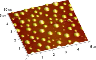
液中に浮遊する直径100 m以下の微細な気泡はファインバブルと呼ばれ，鉱物粒子の選 別[25]や超音波造影剤[26]などその実用化の試みは多岐にわたって展開されており[27]，近 年では直径が1~100 mのものはマイクロバブル，直径1 m以下のものはウルトラファイ ンバブルと国際標準化機構によって定義される[28]など高い注目を集めている．一方で，固 体と液体の界面に存在する非常に薄い気相は界面ナノバブル(Interfacial nanobubbles)と呼ば れている．固液界面ナノバブル(Solid-liquid interfacial nanobubbles)あるいは表面ナノバブル (Surface nanobubbles)と呼ばれることもあるが，その呼称の違いに意味はなくどれも同じも のを指している．そのサイズに厳密な定義はなく，数 m の直径を持つ気泡を界面ナノバ ブルと呼称することもあるが[29,30]，Figure 1.1に示すような直径1 m以下，厚み100 nm 以下のものを指すことが多い．最も多く報告されているのは半球状(Semispherical)ナノバブ ルであるが[5,9,17,19,31–35]，1.2.4節で解説するマイクロパンケーキ(Micropancake)等もまた 界面ナノバブルの亜種として報告されている[17,19,20,32,36–40]．界面ナノバブルは，前述 した通りこれまで説明がつかなかった界面現象を説明しうるのみならず，例えば流動抵抗 の低減[41]やウェハーサイズのグラフェンの転写[42]など，アプリケーションへの応用も期 待されている．

以下の節では，これまでに報告された半球状界面ナノバブルの特性・生成方法・理論につ いて具体的に解説し，近年の計測技術の進歩によって発見されたより厚みが薄い吸着気体 分子層に関する研究を紹介する．

Figure 1.1 Three-dimensional image of interfacial nanobubbles obtained by AFM.

3

1.2.1. 特性

界面ナノバブルが研究対象として脚光を浴びた最も大きな理由は，既存の理論では説明 できないいくつかの特性が発見されたことにある．界面ナノバブルの最初の発見以来，多く の研究者たちがこれらの特性について議論し新たな理論の構築を試みているが，全ての実 験結果を説明できる統一的な理論は未だに存在していない．この節では，これまでに報告さ れた界面ナノバブルの特性について詳細に報告する．

1.2.1.1 接触角

界面ナノバブルの特性の一つとして，形状がマクロな気泡と大きく異なる点が挙げられ る．一般に固体基板上の気泡(あるいは液滴)の接触角 θ は，固体－気体－液体の三相界線

(Three-phase contact line)における水平方向の表面張力の釣り合いを表すYoungの式(1.1)によ

って表される．

𝛾 = 𝛾 + 𝛾 cos 𝜃 (1.1)

γは表面(界面)張力(Surface (interfacial) tension)であり，単位はN/mで表される．また添字の

S，G，Lはそれぞれ固体，気体，液体を表している．また，蒸気を意味するVが気体を表

す添え字として用いられることもよくある．この時，接触角は一般に液体側の角度として定 義され，この論文中においても特別に表記されていない限り液体側の角度として取り扱う．

この表面張力の値はその界面を構成する物質の組み合わせで決定するため，式(1.1)より接触 角は固体－気体－液体の組み合わせによって一意的に決定されることになる．しかし界面 ナノバブルは，マクロスケールの気泡に比べてはるかに大きな接触角を持ち，著しく扁平な 形状をしていることが実験的に確認されている．

これまでに界面ナノバブルが生成された基板のマクロスケールの接触角とナノバブルの

接触角をTable 1.1 にまとめる．全ての基板表面上において，界面ナノバブルの接触角は静

的接触角および前進接触角(三相界線が液相側から気相側に濡れ広がるときの接触角)より もはるかに大きな値を示していることがわかる．この接触角の違いは，Youngの式(1.1)では 説明することができない．この理論と実験の差異を説明するために様々な理論が提唱され ているが，それは1.2.3節で紹介する．

現時点で界面ナノバブル生成の再現性が最も高い基板は高配向性グラファイト(Highly ordered pyrolytic graphite: HOPG)である．この理由について，表面の結晶性および濡れ性の異 なるステップの存在という2つの要素が挙げられる．例えばZhangとMaedaはHOPGとア モルファスカーボン基板上で同じ界面ナノバブル生成プロセスを試している[40]．その結果，

同じ炭素原子で構成された基板であるにも関わらず，結晶性を持つHOPG 上では界面ナノ バブルおよびマイクロパンケーキが生成された一方，アモルファスカーボン上では何も生

4

成されなかった．この結果は結晶性が界面ナノバブルの生成に何らかの影響を与えること を示している．またNishiyamaらは撥水性基板表面に親水性ドメインを作製すると，その近 傍に界面ナノバブルが多く生成され，その寿命も延びることを報告している[43]．HOPG表

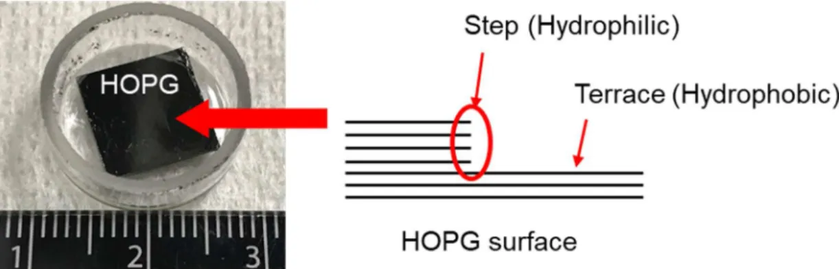
面はFigure 1.2に示すように撥水性のテラス領域と官能基等の修飾によって濡れ性が向上し

たステップ領域で構成されており，親水性のステップ領域が界面ナノバブルの生成を促し ている可能性がある．

Table1.1を見ると，界面ナノバブルはある程度撥水性の表面で頻繁に検出されていること

がわかる．この傾向は固体表面上での不均質気泡核生成を考えるともっともらしい結果と 言える[4]．しかしながら，親水性表面でも界面ナノバブルの生成はいくつか報告されてい る．例えばへき開した雲母(Mica)は非常に濡れ性が良いにも関わらず，いくつもの報告例が ある[5,44,45]．その他にも窒化シリコン[44]や，ガラス[46]といった親水性かつアモルファス な表面においても界面ナノバブルは報告されており，その生成条件に物議を醸している．ま た，親水性基板上の界面ナノバブルは撥水性基板上のものに比べて接触角が小さくなる傾 向が見られるが，例えば前進接触角が85度のHOPG上のナノバブルは160-175度の接触角 を示す一方で，同程度の濡れ性であるZEP膜やより撥水性であるOTS膜付きシリコン基板 上のナノバブルがより小さな接触角を示すなど，基板のマクロスケールな濡れ性と界面ナ ノバブルの接触角の明確な関係性は明らかになっていない．この結果は，ナノスケールの濡 れ性には基板表面のマクロスケールな濡れ性以外の要素が働いていることを示唆している．

Table 1.1 Advancing and receding contact angles of macroscopic water contact angles on various substrates and nanoscopic contact angles of interfacial nanobubbles. All contact angles were determined from water sides. * indicates the static contact angles.

Substrates Advancing (or static*) contact angles [degree]

Receding contact angles [degree]

Contact angles of interfacial nanobubbles

[degree]

HOPG[33,40,44] 85 66 160-175

Talc[40] 67 59 150

Au (111)[47] 40-60* - 126-168

ZEP[48] 89±2* - 147-158

PMMA[48] 63.7±0.4* - 126-150

OTS coated Si[49] 108±5* 150-170

TMCS coated Si[50] 74 67 150-157

PFDS coated Si[51] 105* - 137-164

Silicon nitride[44] 11-13* - 110-130

Mica[5,44,45] 9-13* - 115-155

5

Figure 1.2 A photo of an HOPG and a schematic image of step and terrace structures on an HOPG surface.

6

1.2.1.2 長寿命

EpsteinとPlessetは拡散方程式，ラプラス圧，ヘンリーの法則を解くことでバルク液中に

おける気泡の寿命を求めている[52]．またLjunggrenとErikssonは異なる数学的アプローチ

でEpsteinとPlessetが示したものと同じ結果を導出している[8]．導出の詳細[13]は議論の対

象外であるため省くが，バルク液中で縮小する気泡の寿命は式(1.2)のように表される．

𝑡 ≈ ^{| |}

for large 𝑅 and ζ < 0 for small 𝑅 and any ζ

(1.2)

ここで，𝑅 は初期曲率半径，𝜌 は気体の密度，𝐷は拡散係数，𝑐 は気体の溶解度，ζはガス過 飽和度であり，

ζ = − 1 (1.3)

で定義される．このとき，𝑐 は気泡から十分に離れた位置における気体分子濃度を意味し ている．したがって，ζ > 0は溶存気体の過飽和状態を，ζ = 0は飽和状態を，ζ < 0は不飽和 状態を意味する．ここで𝑅 の”Large”と”Small”は，気泡内部の圧力が大気圧支配かラプラス 圧支配であるかに対応している．Young-Laplaceの式(1.4)から気泡の内圧𝑃は

𝑃 = 𝑃 +

( ) (1.4)

で与えられる．ここで𝑃は大気圧を，𝑅_{( )}は気泡の曲率半径を意味する．この式がナノスケ ールにおいても成り立つことは理論的に証明されている[3]．したがって𝑅( )≫ であれば

式(1.2)中の large 𝑅 に対する式が，𝑅( )≪ であれば式(1.2)中の small 𝑅 に対する式が適

用される．大気圧条件下における純水中の気泡であれば， ≈ 1.4 μmとなるため，一般的 なナノバブルにおいてはsmall 𝑅 に対する式が適用される．その場合，式(1.2)から分かる通 り，ナノバブルの寿命はガス過飽和度ζに寄らず決定する．実際に式(1.2)を用いてナノバブ ルの寿命を計算すると，𝑅 = 10 nmでは𝑡 = 1 μs，𝑅 = 100 nmでは𝑡 = 0.1 msとな り，一瞬で消滅してしまうことになる[8]．また𝑅 = 10 μmを仮定して式(1.2)中の large 𝑅 に対する式を使用した場合でも，気体分子の種類に寄らずナノバブルは数十秒以内に消え

7

てしまうことになる[13]．Ljunggren と Eriksson は式(1.2)による結果から界面ナノバブルは 存在できず，液中に浸漬した撥水性表面間に見られる長距離相互作用の原因を界面ナノバ ブルの懸架によって説明することはできないと結論付けている[8]．

しかしながら，実際の界面ナノバブルの寿命は式(1.2)によって導かれる寿命から大きく逸 脱していることが，数多くの観察実験によって報告されている．例えばZhangらは，Figure 1.3に示すように同じ領域を AFM で計測し続けることによって，いくつかの小さなナノバ ブルは時間経過で溶解する一方，殆どの界面ナノバブルが少なくとも 4 日間以上は存在し 続けたことを報告している[9]．彼らは同時に観察された物体が気相であることを赤外分光 計測によって確認している．

ここで留意すべきなのは，式(1.2)は液中に浮遊する気泡を条件として得られた式であり，

固液界面に存在する気泡に対して適応可能であるかは定かでないことである．実際に界面 に存在する気泡を仮定して得られる式に関しては，1.2.3節で紹介する．

Figure 1.3 Stability of nanobubbles with time at different ambient temperature, where the temperature of liquid is 30 °C: (A) 20 min at 21 °C, (B) 2 days at 21 °C, (C) an additional day at 23 °C, (D) a second additional day at 25 °C (the start of day 5). Some small bubbles dissolved on the third day[9].

1.2.1.3 外乱に対する超安定性

上述した接触角と長寿命に関する特異性は長期に渡って議論されており，それらを説明 する理論は多数存在する．一方，界面ナノバブルの外乱に対する超安定性(Superstability)は，

その奇妙さにも関わらず研究例が限られている．

例えば，Borkentらは界面ナノバブルがキャビテーションの気泡核になり得るかを調べる ため，2 種類の撥水性基板を浸漬した純水に衝撃波を印加し最大で-6 MPa まで急減圧した

[53]．その結果，Figure 1.4に示すように，キャビテーション気泡は基板表面の微小な欠陥あ

るいはコンタミネーションに由来したものしか生成されず，衝撃波の印加後にも界面ナノ バブルが安定して存在し続けていることが明らかになった．彼らは圧力が- 0.55 MPaまで下 がれば曲率半径が100 nmのナノバブルはキャビテーション気泡として成長するはずである と予想していたが，実験結果からは大きく逸脱している．またBrotchieらは界面ナノバブル に超音波を35-40秒間印加し，その前後の界面ナノバブルをAFMによって計測した[54]．

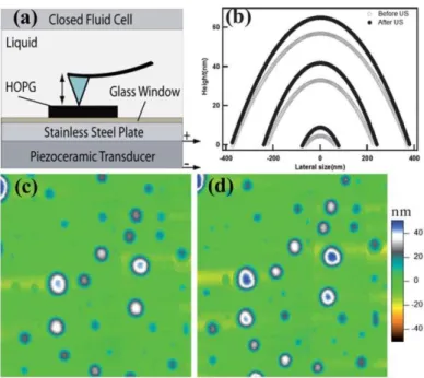
その結果，Figure 1.5に示すように界面ナノバブルは高さ方向への成長が見られた一方，半

8

Figure 1.4 Cavitation activity (left), and corresponding nanobubble density (right) imaged by AFM (topography images) for various probes. The length scales given in (A) also refer to (B), (C), and (D).

(A) and (B): polyamide substrates; (B) after ethanol-water exchange. (C) and (D): hydrophobized silicon substrates; (D) after ethanol-water exchange. There is hardly any cavitation though the substrates are densely covered by surface nanobubbles. Note that the cavitation bubbles in (A) emerge exclusively from microscopic cracks in the surface, whereas the whole substrate is covered by nanobubbles. The cavitation bubbles in (C) presumably originate from surface contaminations[53].

9

Figure 1.5 (a) Schematic representation of the modified closed fluid cell for in situ ultrasound application and tapping-mode AFM imaging; (b) the crosssectional profiles of three pairs of nanobubbles. Tapping mode AFM height images of nanobubbles are shown in (c) prior to sonication and (d) after sonication for 40 s. The scale bars for (c) and (d) are identical and the scan size is 5 × 5

m²[54].

径方向の成長やキャビテーションは観察されなかった．彼らはこの超安定性には固気液三 相界線のピニング(三相界線を特定の位置に固定する現象)が寄与しているだろうと予想し ており，また3次元分子動力学(MD)シミュレーションによって急減圧に対する界面ナノバ ブルの安定性を調査したDockarらも同様の見解を示している[55]．

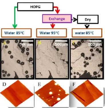
また，界面ナノバブルは周囲の溶液の温度上昇に対しても非常に強力な安定性を示すこ とが報告されている．例えばZhangらは界面ナノバブルが存在する/しないHOPG基板をそ れぞれ沸点近傍まで加熱し，界面ナノバブルが沸騰核として作用するかを調査した[56]．そ の結果，界面ナノバブルが無い場合では85 ℃において気泡が多数生成された(Figure 1.6(a)) 一方，界面ナノバブルがある場合では 95 ℃まで上昇させても気泡が生成されない(Figure 1.6(b))という，直感的な予想に反する結果が得られた．界面ナノバブルの生成に用いた溶媒 交換法が基板表面の性質に恒常的な影響を与えてないか確認するため，基板を乾燥させた のちに純水に再度浸して加熱しているが，やはり85 ℃で気泡が多数確認されている(Figure 1.6(c))．これらの結果は，界面ナノバブルが沸騰核になりえず，むしろその生成を抑制する 方向に作用していることを示しており，撥水性表面における低過熱度での沸騰開始を界面 ナノバブルの存在によって説明するNamとJuの予想[12]を間接的に否定する結果となって いる．また Zhang らはその後，加熱時の界面ナノバブルの挙動を光学顕微鏡によってその 場観察した[29]．その結果，Figure 1.7(a)に示すように界面ナノバブルは90 ℃の液中におい

10

Figure 1.6 Microbubbles nucleated on highly oriented pyrolytic graphite (HOPG) at elevated temperature. (a) Microbubbles formed on HOPG directly exposed to water at 85 °C. (b) After solvent exchange, no microbubbles formed on HOPG at 95 °C. (c) Microbubbles formed again when HOPG was dried after the solvent-exchange process and exposed to water at 85 °C. (d−f) AFM images of HOPG under the same conditions as in a−c, now at room temperature. The area of the AFM images is 5 μm × 5 μm[56].

Figure 1.7 (a) Optical image of nanobubbles in the water phase at 90 °C and (b) the corresponding image of the very same location after the three-phase contact line has passed with microdroplets in the gas phase, with the entrapped nanobubbles. In (b), the temperature is 95 °C. The nanobubbles and resulting droplets are marked with various colors to assist recognition. The patterns of the marks on the surface in (a) are identical to those in (b), demonstrating that all nanobubbles nucleate microdroplets. Also shown are some spontaneously nucleated microdroplets[29].

11

ても安定に存在し続けた．加えて，マクロスケールの気泡の三相界線がナノバブル上を通過 すると，ナノバブルが存在していた場所でマイクロ液滴が生成されることを発見している (Figure 1.7(b))．彼らは，加熱に対する超安定性もまた，三相界線のピニングによってもたら されているだろうと予想している．

これらの超安定性を説明する理論を構築するには，外乱を印加されている最中の界面ナ ノバブルの厚みや内圧の情報が必要不可欠であると考えられる．しかしながら，現時点では，

超音波や加熱は AFM 探針のフィードバック機構に影響を及ぼすため，それらの印加中に AFM計測を行うことは不可能である．ナノスケールの界面気泡が沸騰初期の気泡核生成に 寄与するか否かは沸騰伝熱の分野において重要なトピックであり，例えば計測対象のナノ スケールの厚さ情報を光学的にその場観察できる反射干渉顕微鏡等を用いた，更なる知見 の収集が望まれる．

1.2.2. 生成方法

そもそも界面ナノバブルに関する実験を行うためには，基板表面にナノバブルが存在し ていなければならない．しかし，報告例[6,57]はあるものの，ただ基板を純水に浸漬するだ けではナノバブルはほとんど生成されない．これまでにいくつかの生成方法が考案されて いるが，残念ながら100%の再現性を担保する方法は未だに存在しない．基板表面の濡れ性 や構造が界面ナノバブルの生成に影響を与えるという例もいくつか報告されているが [43,48,58–61]，待ち望まれているのはどのような基板表面においても確実に生成されるよう な手法である．この節では，これまでに報告された代表的なナノバブルの生成方法について 紹介する．

1.2.2.1 溶媒交換法

溶媒交換法(Solvent exchange method)は，界面ナノバブル生成に最初に用いられた方法で あり[5]，また最も頻繁に用いられる方法である．この方法には一般にエタノールと水が用 いられ，それらの溶液の気体の溶解度が大きく異なることを利用している．まず，基板をエ タノールに浸漬させて数分待つ．その後，注射器等で純水をゆっくり注入することで，エタ ノールと純水を置換する．エタノールは水に比べて気体の溶解度が高いため，この置換過程 で液中に一時的な気体の過飽和状態が生じる．その結果，基板表面付近の余剰な気体分子に よって，界面ナノバブルの生成が促される．

溶媒交換法の利点は，手順が単純なことである．気体の溶解度の差を利用した方法であり，

空気中に暴露されている溶液は一般に空気を飽和状態まで溶解しているため，バブリング 等の特別な工程を必要としない．逆に言えば，エタノールと水を十分に脱気すると，界面ナ ノバブルはほとんど生成されなくなる[57]．また，エタノールと水に特定の気体のみを溶解 させておけば，その気体で構成されたナノバブルを生成することも可能である[9]．さらに，

12

水の代わりにホルムアミドのような有機溶媒や硝酸エチルアンモニウムといったイオン液 体を用いた場合[62]や，エタノール以外にメタノールやプロパノールといった他の有機溶媒 を用いた場合[63]でも溶媒交換法が成功することが確認されている．

溶媒交換法は界面ナノバブル生成に最も頻繁に用いられている方法であるが，いくつか の問題点も存在する．例えば，必ず二種類の液体を混ぜるため，一つ目の溶液を完全に置換 しきれず混合溶液になっている可能性がある．そうすると表面張力の値が変わってしまい，

界面ナノバブルの形状や性質に変化が生じうる．Zhangらは溶媒交換法後に水槽内の溶液の 化学成分をガスクロマトグラフィーと質量分析装置で分析し，エタノールが残留していな いことを確認している[64]．また，置換中の流速や流量，流れの方向，液体の温度など，ナ ノバブル生成に関わるであろういくつかの重要なパラメータがどれも詳しくは報告されて いない．そのため各実験において実験条件がまちまちであり，再現性の低下の要因となって いる．また最近の報告で，医療用にも用いられる使い捨ての注射器を用いて溶媒交換法を行 うと内部に塗布された痛み軽減用の潤滑剤に由来するナノ液滴が生成されることがわかっ た[22]．このナノ液滴は界面ナノバブルにそっくりの形状をしており，識別が難しい．した がって，信頼性向上のために，溶媒交換法は潤滑剤などが塗られていない金属製の注射針や ピペット等を用いて行うべきである．

溶媒交換法を拡張した方法として，温度差法がある[65]．この方法は気体の溶解度の温度 依存性を用いたもので，基板を冷たい水(4 ℃)に浸漬させた後に温かい水(25-40 ℃)で置換す ることでナノバブルを生成する．置換過程で生じる気体の過飽和状態を利用する点は溶媒 交換法と同じであるが，この方法の利点は，純水のみを使うことができるために有機溶媒由 来のコンタミネーションの可能性を排除できることである．しかし，依然として置換におけ る流れのパラメータは考慮されておらず，再現性に疑問が残る．

1.2.2.2 マイクロ波照射

マイクロ波照射によるナノバブル生成は最近考案された方法である．溶液に浸漬した状 態の基板を調理用電子レンジに入れ，任意の出力・照射時間でマイクロ波を照射することで ナノバブルを生成する．

Wangら[66]は，酸素を飽和状態以上まで溶解させた純水中にHOPG基板を浸漬させてマ イクロ波を照射した(Figure 1.8(a))．その結果，照射時間(Figure 1.8(b))，作動出力(Figure 1.8(c))，

初期溶存酸素量(Figure 1.8(d))をそれぞれ増加させることで，界面ナノバブルの生成個数が増 加することがわかった．彼らはこの方法でナノバブルが生成される原理として，マイクロ波 加熱による温度上昇によって気体の溶解度が急速に下がるという熱的効果と，電界の正負 方向の変化に合わせて水分子が高速で振動するため水分子－酸素分子間の水素結合が切れ やすくなるという非熱的効果の二つを挙げている．

この方法では純水のみを用いるため，有機溶媒由来のコンタミネーションのリスクがな くなることに加え，溶媒の置換に起因する流れを考慮する必要がなくなるため実験の再現

13

性が高い．現状ではWang らによる HOPG 基板と酸素飽和純水を用いた実験しか報告され ていないが，異なる基板や，異なる気体を溶解させた溶液を用いても同様にナノバブルが生 成できるならば，溶媒交換法に取って代わる有力な生成方法になりうる．

Figure 1.8 (a) Schematic diagram of nanobubble generation via microwave. Effect of (b) microwave irradiation time, (c) microwave power, and (d)dissolved oxygen concentration on the formation of nanobubbles[66].

1.2.2.3 電気分解

水の電気分解によって陽極・陰極表面にそれぞれ酸素・水素のナノバブルが生成されるこ とが，実験的に確認されている．このとき，電圧の印加を止めてもナノバブルは安定に存在 し続けるため，容易に計測を行うことができる．この方法には，導電性の表面しか試料表面 として使えないことや，ナノバブルを構成する気体の種類が制限されるなどの欠点が存在 する．さらには，電圧印加時の界面ナノバブルの正確な挙動が現在まで分かっていない．

Zhangら[67]は電圧の印加時間に比例してナノバブルは成長し続けると報告している一方で，

Yang ら[68]はナノバブルが成長するのは一定の時間のみでありそれ以降は電圧を印加し続 けても成長しないと報告している．この相反する結果は実験条件の差によるものと考えら れる．例えば，Zhangらは溶液として脱気した0.01 M 硫酸を用いているが，Yangらは未脱 気の純水を用いている．また，両実験とも電極(HOPG)の表面積が大きすぎるため電極表面

14

の電界分布が不均一になり，局所的なナノバブルの生成に影響を与えた可能性も考えられ る．

電気分解法では，電極の表面積を非常に小さくすることで界面ナノバブルの生成速度を 精密に計測あるいは制御できる可能性がある．Whiteら[69–73]は直径50 nm未満のナノディ スク電極を作製し，その表面に単一のナノバブルを生成することに成功している．このよう な電極は，単一ナノバブルの物理を理解するのに大いに役立つ．例えばWhiteらは，電流電 圧の時系列データから電極近傍のガスの濃度分布やナノバブルの表面張力などが推定でき るとしている．

1.2.3. 理論

前述した通り，界面ナノバブルにはいくつもの未解明の物理が存在する．特にその極端に 大きな接触角と長寿命に関しては，既存の理論で得られる結果から大きく外れていること から，それらを合理的に説明できる理論の確立に多くの研究者が挑戦している．その努力は 現在も続いているが，未だに全ての実験結果を矛盾なく説明できる理論は存在していない．

この節では，これまでに報告された理論の中で最も有名な3つの理論を紹介するとともに，

それらの理論が孕む問題点についても指摘する．

1.2.3.1 コンタミネーション理論

コンタミネーション理論は，Ducker によって提唱された界面ナノバブルの接触角と長寿 命を説明する最初の理論である[74]．彼は，ナノバブルの気液界面に形成される不溶性のコ ンタミネーション層が安定化の要因であると説明した．具体的には，コンタミネーションの 付着によって気液界面の表面張力は低下し，接触角と曲率半径が増加する．その結果，式 (1.4)から分かる通り，液中へのガス拡散の駆動源であるラプラス圧が減少する．また，不溶 性のコンタミネーション層はナノバブルから液中へのガス拡散を物理的に妨げる．さらに，

気液界面はガス拡散が進行するにしたがって小さくなるため，コンタミネーション層はよ り厚くなりナノバブルを安定化させる．

この理論は現在ではいくつかの実験結果から否定されることが多い．例えば，Zhang ら [75]は界面ナノバブルの生成後に十分な濃度の界面活性剤を液中に添加し，気液界面の有機 物をすべて取り除くことで界面ナノバブルの安定性が変化するか調査した．その結果，界面 活性剤の添加前後で界面ナノバブルに変化はほとんど見られなかった．さらに，コンタミネ ーションを模擬した不溶性の界面活性剤(オレイン酸)を添加した場合，界面ナノバブルは生 成されなくなった．これらの結果は，コンタミネーション理論と大きく矛盾している．次に，

界面ナノバブルはナノバブル同士で合体することが知られている．Agrawalら[61]はAFM計 測中，計測モードにおける種々のパラメータの設定値によってはナノバブル同士が合体す ると報告した．また，気液界面や三相界線が接触することなく，小さなナノバブルが大きな

15

ナノバブルに液相を通じて吸収される現象(オストワルドライプニング)も報告されている [76,77]．ナノバブルの気液界面が不溶性のコンタミネーションで覆われているとすると，こ れらの合体は起こりえない．最後に，Zhang ら[9]は界面ナノバブルを構成する気体によっ て，ナノバブルの寿命が変化することを発見した．空気で構成されたナノバブルは4日間安 定して存在し続けた一方，二酸化炭素で構成されたナノバブルは1-2時間で消滅した．コン タミネーションが気液界面を覆うことで気体分子の流出を防いでいるならば，気体の種類 による寿命の違いは大きくないはずである．これらの結果より，現在ではコンタミネーショ ン理論による界面ナノバブルの安定性の説明は不十分であるとされている．

1.2.3.2 動的平衡理論

撥水性基板と水の界面には水分子の数密度が低い領域が存在し，そこに溶存気体が蓄積 することでガスエンリッチメント層[78–83]が形成されている．Brennerらは，ラプラス圧に よって液中に拡散される気体の外向き流束とガスエンリッチメント層から三相界線近傍を 通じて流れ込む気体の内向き流束が釣り合うことで界面ナノバブルが動的に安定している と提唱した[84]．Figure 1.9(a)に動的平衡理論の概念図を示す．導出は省くが，拡散方程式を 解くことで内向きの体積流量𝑗_inと外向きの体積流量𝑗_outはそれぞれ以下のようになる．

𝑗 =2𝜋𝑠𝐿𝐷

tan 𝜃 (1.5)

𝑗 = 𝜋𝑟𝐷 1 −

( ) (1.6)

これらの式において，𝐷は気体の拡散係数，𝐿は界面ナノバブルのフットプリント半径，𝑠は 固体表面からの引力の強さを表す定数，𝜃は気相側の接触角，𝑐 は界面ナノバブルから遠方 での気体分子濃度，c(𝐿) = 𝑐 は界面ナノバブル表面での気体分子濃度，𝑐 は大気圧𝑃 下 での気体分子の飽和濃度，𝑃 はラプラス圧である．式(1.5)と(1.6)をプロットした図[84]を

Figure 1.9(b)に示す．𝐿がある値𝐿^∗よりも小さいと 𝑗 が𝑗 よりも大きくなるため𝐿は大きく

なり，𝐿^∗よりも大きい場合は逆に𝐿は小さくなる．最終的に，界面ナノバブルは𝑗 と𝑗 が釣 り合う平衡フットプリント半径𝐿^∗を維持することになる．

いくつかの界面ナノバブルの挙動や実験結果は，この動的平衡理論によってうまく説明 できる．まず，脱気した水中では界面ナノバブルが消えてしまうという現象が説明できる

[22,85]．脱気した水中では𝑐 が減少するため，式(1.6)より外向き流束が増加する．また，内

向き流束は撥水性基板表面近傍の気体分子密度に由来している．脱気水中ではその密度が 低下し，内向き流束が減少していると予想される．その結果，正味の外向きガス拡散が増大 し，ナノバブルは消滅する．液温が上昇するとナノバブルの体積が増加する理由も説明でき

16

る[51]．温度が上昇するにつれて𝑐0が減少するため，それに従って𝑐(𝐿)も減少する．その結 果，式(1.6)より外向き流束が減少する．さらに，温度上昇に伴って撥水性表面の水分子密度 が低い層の厚みが増加することが実験によって報告されており[79]，そのため内向き流束の 増加が予想される．したがって，温度が上昇すると正味の内向きガス拡散が大きくなり，バ ブルの体積は増加する．

しかし，動的平衡理論では説明できない謎も残されている．たとえばZhangらは，代表的 な親水性基板であるマイカ表面にナノバブルが存在することを確認している[85]．この理論 では撥水性表面上にあるガスエンリッチメント層の存在が界面ナノバブルの安定性の前提 となっているため，親水性表面のナノバブルの安定性を説明できない．Yasuiらは界面ナノ バブル中の気体分子と固体表面間に働くファンデルワールス力を考慮することによって，

親水性表面のナノバブルの安定性を説明できるよう動的平衡理論を拡張している[86]．また，

動的平衡理論では界面ナノバブルのフットプリント半径𝐿^∗は実験条件によって一意的に決 定されるが，実際のフットプリント半径は不均一に分布している．これは，この理論が理想 的に平滑な基板表面を仮定して構築されているからだと考えられている．実際の基板表面 では，ピニングと呼ばれる表面の構造的・化学的不均一に由来して三相界線を固定する現象 が起こるため，フットプリント半径が理論値からずれる．動的平衡理論をさらに発展させるには，

Figure 1.9 (a) Schematic picture of dynamic equilibrium theory. (b) Gas outflux 𝑗 and influx 𝑗 into the surface nanobubble as function of bubble radius R. The crossing point defines the equilibrium footprint radius L. The units of 𝑗 are m /s. If the slope of 𝑗 at L = 0 is larger than that of 𝑗 , no surface nanobubbles can emerge. The detailed data to illustrate this plot is written in [84].

17

三相界線のピニングによる影響を考慮する必要があるだろう．加えて，Dietrichらは粒子ト ラッキング解析によって動的平衡理論で予測される界面ナノバブル周辺の流れの観察を試 みたが，界面ナノバブルの有無で粒子の挙動に違いは無かったと報告している[87]．

1.2.3.3 ピニングとガス過飽和

固気液三相界線のピニングは，界面ナノバブルの性質を語る上で欠かせない要素である．

特にその長寿命には，ピニングが密接に関わっているとされている．例えば，界面ナノバブ ルの三相界線がピニングされていると仮定すると，フットプリントは一定に維持される．し たがって，ナノバブルが縮小する時は高さのみが減少するため，曲率半径が大きくなる．そ の結果，拡散の駆動源となるラプラス圧が低下し，外向きガス拡散は抑えられる．逆に，ナ ノバブルが成長する時は高さのみが増加するため曲率半径は小さくなる．そのためラプラ ス圧が上昇し，外向きのガス拡散量は増加する．このように，ピニングはナノバブルの体積 変化に対してネガティブフィードバックをかけ，常に安定性を高める働きをする．

界面ナノバブルの三相界線が実際に強くピニングされていることは，多くの研究によっ て実験的に明らかになっている．例えば Brotchie らは超音波の印加によって界面ナノバブ ルが成長する際，高さ方向にのみ成長し三相界線の位置はほとんど変化しなかったことを 報告している(Figure 1.5)[54]．またZhangらは，溶媒交換法で界面ナノバブルを生成した水 中に脱気水を加えることで，ガス飽和度が低い純水中でのナノバブルの形状変化を観察し た[31]．その結果，いくつかのナノバブルはすぐに消滅し，残ったナノバブルも 14 時間以 内に縮小するか消滅した．その過程で，ナノバブルの三相界線が強くピニングされているこ とを報告している．またこの結果は，界面ナノバブルの長寿命にはピニングと同様に液中の 溶存ガス濃度が重要であることを強く示している．

2015 年，Lohse とZhang は三相界線が強くピニングされることでフットプリント半径が 変化しない単一の界面ナノバブルを仮定することで，古典的な理論(拡散方程式・ラプラス 圧・ヘンリーの法則)のみを用いて界面ナノバブルの平坦な形状と長寿命を説明した[88]．ま ず彼らは，Popovが導出したコーヒーステイン現象によって三相界線が固定された液滴の蒸 発に関する式[89]を拡張することで，三相界線が固定された界面ナノバブルの質量𝑀(𝑡)の時 間変化率を式(1.7)のように求めている．

𝑑𝑀 𝑑𝑡 = −𝜋

2𝐿𝐷 𝑃 +4𝛾 sin 𝜃 𝐿

𝑐

𝑃 − 𝑐 𝑓(𝜃) (1.7)

ここで𝑓(𝜃)は

𝑓(𝜃) = sin 𝜃

1 + cos 𝜃+ 4 1 + cosh 2𝜃𝜉

sinh 2𝜋𝜉 tanh[(𝜋 − 𝜃)𝜉] 𝑑𝜉 (1.8)

18

であり，常に正の値である．また式(1.7)において，𝐿は界面ナノバブルのフットプリント直 径であり，𝜃は界面ナノバブルの気相側の接触角である．さらに，気泡の密度をρ とすると，

気泡の体積𝑀(𝑡)は幾何的に式(1.9)のように表すことができる．

𝑀(𝑡) = ρ 𝜋

8𝐿 cos 𝜃 − 3 cos 𝜃 + 2

3 sin 𝜃 (1.9)

式(1.7)と式(1.9)から，気相側の接触角𝜃に関する常微分方程式は式(1.10)のように得られる．

𝑑𝜃

𝑑𝑡 = −4𝐷 𝐿

𝑐

ρ (1 + cos 𝜃) 𝑓(𝜃) L

𝐿 sin 𝜃 − 𝜁 (1.10)

ここで，L = は定数(2.84 m)であり，𝜁は式(1.3)と同じ定義で与えられるガス過飽和度

である．

式(1.10)から，不飽和状態(−1 ≤ ζ < 0)の液中では右辺が常に負になるため接触角が減少し 続け，界面ナノバブルは安定に存在できないことがわかる．これは脱気水中では界面ナノバ ブルが消滅するという実験結果と一致している[22,85]．しかしながら，過飽和状態(ζ > 0)の

液中では = 0を満たす平衡接触角𝜃 を持つ界面ナノバブルが存在することができ，その接

触角の値は式(1.11)で与えられる．

sin 𝜃 = 𝜁 𝐿

𝐿 (1.11)

上式の通り，界面ナノバブルの形状はガス過飽和度𝜁の値によって一意的に決定されるため，

Figure 1.10(a)に示すように界面ナノバブルが初期接触角𝜃を持っていようとも𝜃 に徐々に変

化し，平衡状態となる．また式(1.11)から得られるFigure 1.10(b)を見るとわかるように，液 中のガス過飽和度が高いほど平衡接触角が大きくなることがわかる．

この理論とEpsteinとPlesset[52]およびLjunggrenとEriksson[8]が導出した理論はどちらも 同様に古典理論のみを用いているが，大きな違いは液中に浮遊する気泡ではなく固液界面 の気泡を仮定し，その三相界線が強くピニングされているとしたことである．その後Dollet

と Lohse はこの理論を 2 つの界面ナノバブルが存在する場合に拡張し，サイズが違う気泡

間で起こり得るオストワルドライプニングがピニングによって抑制されることを理論的に 示した[90]．

19

この理論は，ピニングとガス過飽和度という経験的に重要だと考えられていた要素を巧 みに理論に取り込んでいることから，界面ナノバブルの性質を今のところ最も上手く説明 できているとされている．しかし，この理論にもまだ問題は存在している．基板の濡れ性と 接触角の関係が実験結果と一致しない点である．界面ナノバブルの気相側の接触角は，基板 表面が親水性になるにつれて大きくなる傾向があると実験的に報告されており[44]，また

Table 1.1からも読み取れるのに対して，基板表面の親水性が強まるとガス過飽和度𝜁は低く

なると考えられるため，Figure 1.10(b)が示すガス過飽和度が低くなるにつれて気相側の接触 角が小さくなるという結果は矛盾してしまう．また現時点では界面ナノバブル付近のガス 過飽和度𝜁を定量的に測定する手法が存在しないため，この理論の定量的な厳密性を議論す ることはできない．

Figure 1.10 (a) Sketch of the shrinking process of a pinned surface nanobubbles with initial contact angle 𝜃: Due to the pinning, footprint is fixed. Shrinking thus implies a decrease in 𝜃 and height and an increase in the radius of curvature. Therefore, the Laplace pressure inside the bubble reduces and eventually becomes too weak to further press out the bubble against the oversaturation. (b) Equilibrium contact angle 𝜃 of a nitrogen bubble in water as function of the lateral footprint diameter L for four different oversaturations 𝜁 = 0.25, 0.5, 1.0, 2.0, bottom to top[88].

1.2.4. より厚みが薄い吸着気体分子層

これまでの節では，半球状の形状を持つ界面ナノバブルについて紹介してきた．しかしな がら，固液界面には界面ナノバブルよりも薄く扁平な気相が吸着しており，しかも構造的特 徴の異なる数種類が存在することがAFM計測によって明らかになっている．特に1.2.4.2節 で紹介する整列層と非整列層は発見から日が浅く，真の疎水性相互作用[10,14]に代表される これまで未解明であった物理を紐解く一助になるのではないかと期待されている．この節 では，これまでの界面ナノバブルよりも厚みが薄い気相の報告例とその性質を紹介する．

20

Figure 1.11 Micropancakes and nanobubble-pancake composites formed after solvent exchange method: (a) height image, (b) section of the height image, and (c) phase image of micropancakes; (d) height image, (e) section of the height image, and (f) phase image of nanobubble-pancake composites[38].

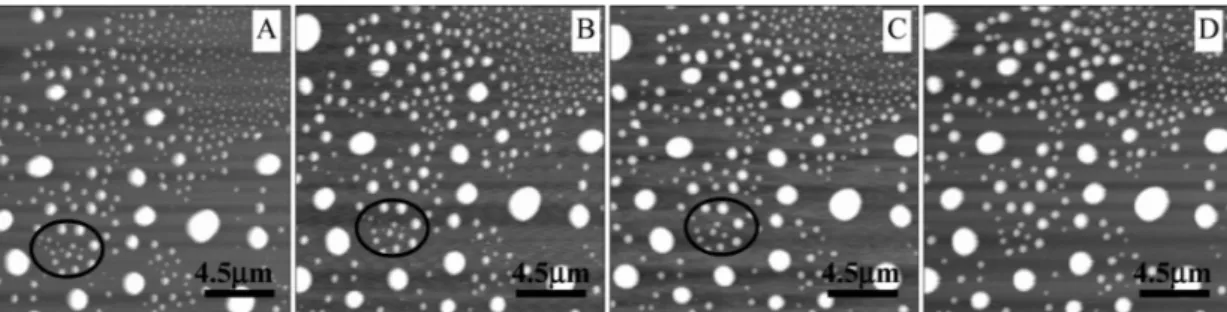
Figure 1.12 Change of micropancakes and nanobubbles as a function of time and temperature: (a) initial pancakes (P = micropancake) immediately after the displacement of ethanol with water at 31 ± 0.5 °C; (b) after 1.5 h at 31 ± 0.5 °C, P1 and P2 coalesced into a bigger micropancake, P3 (the nanobubbles on the micropancakes could move with time, for example, the one inside the dotted circle); (c) after another 1.5 h at this temperature, the pancakes are not very different from those in image b; (d) recommencement of growth of P3 if the temperature is increased to 36 ± 0.5 °C and held for 0.5 h[38].