密度成層流体中の物体により励起される3次元非線形内部重力波:Navier-Stokes方程式の解と外力項を持ったKP方程式の解(流体における波動現象の数理とその応用)

(1)

密度成層流体中の物体により励起される

3 次元非線形内部重力波

-Navier-Stokes

方程式の解と外力項を持った

KP

方程式の解

–

国立環境研究所 _花崎秀史 (Hideshi HANAZAKI)

1.Introduction

Recent studies

on

the

waves

excited by

an

obstacle in the flow have revealed the basic nonlinearwave-generationmechanism. The mechanism is

now

found tobe essentially the

same

for the water waves, internal gravity

waves

in stratified flows and for the inertial

waves

in swirling flows. The two-dimensional

waves

excited

near

resonance are

foundto

be well described by the forced Boussinesqequation

or

the forced $KdV(fKdV)$equation.

Thesemodel equations have been derived by Wu(1981) andAkylas(1984) for the water

waves, by Grimshaw&Smyth(1986) for the internalwaves, and by Grimshaw(1990) for

the swirling flows. The applicability of these equations and their extensions has been verifiedexperimentally

or

numerically byLee,Yates&Wu(1989) forthe waterwaves, by

Zhu,Wu&Yates(1986),

Melville&Helfrich(1987)

and Hanazaki(1992) for the internal

waves, and Hanazaki$(1991, 1993a)$ for the swirling flows.

However, for the three-dimensionalwaves, sufficient results have not been obtained. In

an

experiment for the water wave, Ertekin,Webster&Wehausen(1985) found that the

upstream

waves

become straight crested. To know the applicability of the weakly

nonlinear theories, Ertekin,Webster

&Wehausen(1986)

solved the Green-Naghdi

equation, Katsis

&

Akylas(1987) solved the forced KP(fKP) equation and

Pedersen(1988) solved the forcedBoussinesqequation. They foundthat,

near

resonance,

upstream

waves

become two-dimensional and the generationperiod of theupstream

wave

agrees

withexperiments. From theirresults, Katsis&Akylas(1987) andPedersen(1988)

argued that the mechanism of the two-dimensionalisation is the Mach reflection of the

upstream

waves

at the side wall ofthe channel. However, _{Tomasson&Melville(1991)}

solved

an

equation for the

waves

excited by

a

side wall perturbation in the two-layer flow. Theequation is similartothe $fKP$equation, and with

an

additional assumption [see their (21)] itbecomes the$fKP$equation. Because the solution of thatequationagreedwell with the solution of the linearized version of that equation when the flow is subcritical,

they argued that the phenomenon

can

be explained by the differences in the

group

velocity ofthe lateral modes of the linear

wave.

Since

no

experimental results exist that

can

follow the time development of the three-dimensionalpatterns of the upstream wave,

quantitative verification of the $fKP$

or

the forced Boussinesq equations

as a

time-dependent weakly nonlinearmodelhasnotbeen done sufficiently.

For the

waves

in

a

flow of linearly stratified Boussinesq fluid, there

are a

number of

experiments, but

none

of these givethree-dimensionalperspective of the upstream

wave.

Hanazaki(1989a) has found that theupstream

waves

become two-dimensional by solving

thethree-dimensional Navier-Stokes equations.However,the channel width used

was

too

small forthe understanding oftheprocess of the two-dimensionalisation of theupstream

(2)

for the two-dimensional resonant flow and its quantitative verification

was

done numerically by Hanazaki(1993b). However, corresponding theory for the three-dimensional

waves are

notyetdeveloped. Because the linearly stratified Boussinesq fluid

is

one

of the most typical type of density stratification that has been studied extensively, the investigationof its three-dimensional flowis also of much interest.

In this study, time-dependent three-dimensional Navier-Stokes equations

are

solved numerically. First,

near

resonant flow of the nearly two-layer fluid is considered. It is

shown if the

waves

resonantly excited by

an

obstacle

are

describable by the equations

derived by the weaklynonlinear theory andifthe abnormal reflection similartothe Mach reflection

occurs

atthe side$waU$ and also ifthe

process

oftwo-dimensionalisationof the

upstream

waves

can

be explained by the differences in the

group

velocity of the lateral

modes of the linear

wave.

Inthiscase, the

waves are

expectedtobe governed bythe $fKP$

equation

or

its extensions and the comparisons with their solutions

are

given. Next, the results for the flow of the linearlystratified Boussinesq fluidis given.

2.$Theory$

Thegoverning equations

are

theNavier-Stokesequations for

an

imcompressiblestratified fluid.

$\frac{\partial_{\mathcal{V}}^{\vee}}{\partial r}+(varrow\cdot\vec{\nabla})\vec{v}=-\frac{1}{\rho}\vec{\nabla}p-g^{\wedge}zarrow+\frac{\mu}{\rho}\nabla^{2}\vec{v}$, (2.1a)

$\frac{\partial p}{\partial t}+(varrow\cdot\tilde{\nabla})p=0$, (2.1b)

$divv=0$ (2.1c)

where $\vec{v}=(u,v,w)$ is the velocity, $p$ is the

pressure,

$r$ is the density, $m$ is the viscosity

coefficient, $g$is the acceleration duetogravityand

$\overline{z}\wedge$

is theunitvectoralong the$z$ axis.

To derive the forced KP(fKP)equationand the forced extendedKP(flEKP) equationffom the inviscid form of(2.1),

we

rescale

x,y

and $t$

as

$X=\epsilon^{1/2}x,$$Y=q,$$T=\epsilon^{3/2}r$_, (2.2)

where $\epsilon$ is

a

smallparameterand expand the dependentvariables in

powers

of $\epsilon$

.

At $O(\epsilon)$,

we

obtain

a

Sturm-Liouville equation

$\frac{d}{dz}(\overline{\kappa}_{n}^{2}\frac{d\phi_{n}}{dz})-g\frac{d\overline{p}}{dz}\phi_{n}=0$,

$\}_{2.4}^{2.3}\{$

$\phi_{n}(0)=\phi_{n}(D)=0$,

where $C_{n}(C_{1}>C_{2}>\ldots)$ and $\phi_{n}(z)$

are

respectively the nth eigenvalue and the nth

eigenfunction and $\overline{p}(z)$ is the undisturbed density.

If

we

scale the obstacle height$h$

as

$h=\epsilon^{2}H(X,Y,T)$_, (2.5)

we

obtain the $fKP$ equation at $O(\epsilon^{2})$, and if

we

consider also the effect of the cubic

nonlinearity of higherorder,$O(\epsilon^{3})$,

we

obtain the$fEKP$equation

$- \frac{1}{C_{\hslash}}(A_{T}+\Delta A_{X})+a_{7}AA_{X}+\epsilon a_{2}A^{2}A_{X}+a_{3}A_{XXX}+\frac{1}{2}\int_{-\infty}^{X}dKA_{YY}+G_{X}=0$, (2.6)

(3)

$\Delta=\frac{U-C_{n}}{\epsilon}$, (2.7a) $a_{1}= \frac{3\int_{0^{D}}\overline{\rho}(\frac{d\phi_{n}}{dz})^{3}dz}{2L_{\hslash}}$ , (2.7b) $a_{2}= \frac{3\int_{0^{D}}\overline{\rho}(\frac{d\phi_{n}}{dz})^{4}dz}{L_{n}}$ , (2.7c) $a_{3}= \frac{\int_{0^{D}}\overline{\rho}\phi_{\hslash}^{2}dz}{2L_{\hslash}}$ , (2.7d)

$G(X,Y)=( \overline{\rho}\frac{d\phi}{dz})_{z=0}\frac{H(X,Y,T)}{2L_{n}}$, (2.7e)

and $L_{\hslash}= \int_{0^{D}}\overline{\rho}(\frac{d\phi_{n}}{dz})^{2}dz$

.

(2.7f)

The$fKP$equation is obtained by neglecting the cubic nonlinearterm $\epsilon a_{2}A^{2}A_{X}$ in(2.6). In

a

two-dimensional two-layerflow,

Melville&Helfrich(1987)

found by experiments that

the effect of the cubic nonlinearity cannot be neglected. Later, Hanazaki(1992) showed that theratio $\epsilon a_{2}/a_{1}$ is

very

large compared tothe

case

of thewater

wave

and the

waves

would be well described by the $fKP$ equation only when the amplitude of the

wave

is

very

small.In the

case

of the linearly stratified Boussinesqfluid, (2.3)becomes

$\frac{d^{2}\phi_{\hslash}}{dz^{2}}-\frac{N^{2}}{C_{\hslash}^{2}}\phi_{\hslash}=0$, (2.8a)

where the constantBrunt-Vaisala frequency isgiven by

$N^{2}=- \frac{g}{\overline{p}}\frac{d\overline{\rho}}{dz}$

.

(2.8b)

Therefore, $\phi_{\hslash}(z)$ and $C_{n}$become

$\phi_{n}(z)=\sin\frac{n\pi z}{D}$, (2.9a)

and

$C_{n}= \frac{ND}{n\pi}$

.

(2.9b)

Substituting (2.9a) into ($2.7b,f\gamma$ and setting $\overline{\rho}(z)$

constant in the integrand,

we

know that

$a_{1}=0$, which

means

that the quadratic nonlinearterm in the $fKP$and the $fEKP$ equation

vanishes. In this

case

the nonlinear correction of the linear

wave

speed would be

very

small. This

can

be expected from the solution of the equation derived by Grimshaw&

Yi(1991) and from the numerical solution of the two-dimensional Navier-Stokes

equations [Hanazaki(1992,1993b)].

3.Numerical method

The numerical method is essentially the

same as

in the previous

studies[Hanazaki(1989a,b),(1992)]. The computation

was

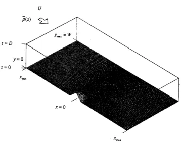
done in the domain of

(4)

where$W(=40D)$is the half width ofthechannel,$D$ is thechannel depth and the obstacle

shapeis given by

$h(x,y)=h_{m*x} \cross\frac{1}{2}[1+\cos(\pi\{(\frac{X}{5D})^{2}+(\frac{y}{10D}I^{2}\}^{\frac{1}{2}}]]$,

where $( \frac{X}{5D})^{2}+(\frac{y}{10D}I^{2}\leq 1$ (3.2)

and $h(x,y)=0$elsewhere [$h_{mx}=0.1D$,

see

Figure 1].

The computation is done only for $y\geq 0$ because

we assume

the symmetry of the flow against the plane of $y=0$

.

_At $y=W$ and $z=D$, _{rigid walls} _exist _{and the}

_waves

are

reflected by these walls. The boundary conditions for the nearly two-layer flow

are

the three-dimensional counterpartoftheprevious studies [Hanazaki(1989a,b), (1992)].

Theundisturbed density distribution $\overline{p}(z)$ is givenby

$\overline{p}(z)=\frac{1}{2}[\overline{\rho}(0)+\overline{\rho}(D)]-\frac{1}{2}[\overline{\rho}(0)-\overline{\rho}(D)]\tanh[\frac{50(z-f_{b})}{D}]$,

(3.3)

with $\overline{\rho}(D)=0.9\overline{p}(0)$, and _{$h_{2}=0.3D$}

.

Inthis study, Froude numberis defined by

$F= \frac{U}{C_{1}}$

.

(3.4)

where $C_{1}$ is the maximum eigenvalue of the Sturm-Liouville problem (2.4). Specifically,

in the

case

of the linearly stratified Boussinesq fluid, $C_{1}$ is given by (2.9b) (with $n=1$).

The Froudenumberisvaried

as

$0.6\leq F\leq 1.4$

.

The Reynolds numberisdefined by

${\rm Re}=^{\underline{\overline{\rho}(0)Uh_{\max}}}$

.

(3.5)

$\mu$

andis fixedtobe

1000.

4.Results

In Figure 2, time development of the resonant(F$=1.0$) flow of

a

nearly two-layer fluid

over

topographyisdescribed. Here $A(x,y,t)=Al$(x,y,t) is calculatedusing the horizontal

velocity $u(x,y,z,t)$

.

In the initial time development(Ut/D$=40$) the upstream

waves

are

curved backwards [Figure $2(a)$]. At around $Ut/D=60$, the far side end of the upstream

waves

reaches the side wall anditbegins tobe reflected. Afterthat, the upstream

waves

become gradually straight crested

as

time proceeds. Downstream of the obstacle, flat depression is formed andit becomes longer

as

timeproceeds. Further downstream, lee

waves

are

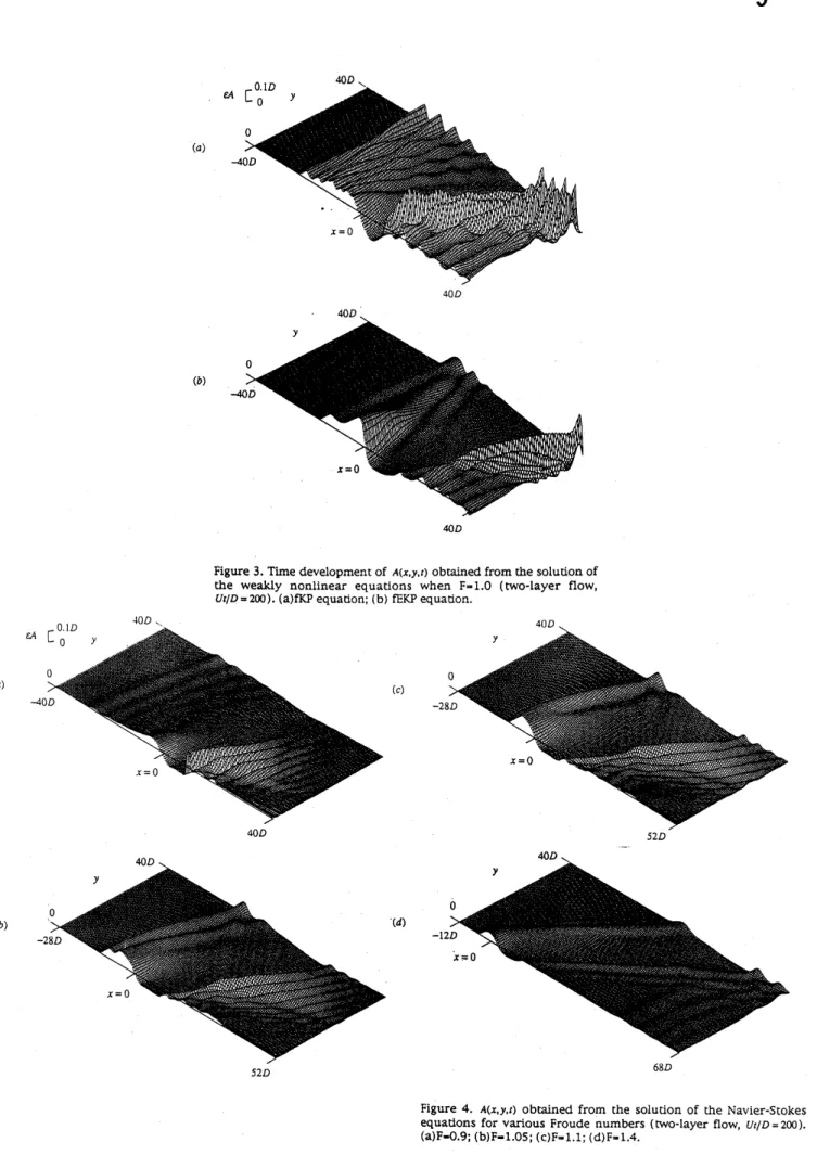
generated[Figure$2(d)$].

To

compare

this solution with the weakly nonlinear theory, the solutions of the$fKP$ and the $fEKP$ equation [see (2.6)] when$F=1.0(UUD=200)$

are

_{shown in Figure}

3.

_The

over

all qualitative feature agree with the solution of the fully nonlinear Navier-Stokes

equations. However, there

are

some

quantitative differences. Nearly flat depressionjust downstream ofthe obstacle(x$>0,$$y\equiv 0$), whichis typical in the two-dimensional

waves

and also

seen

in the three-dimensional solution of the Navier-Stokes equations, does not

(5)

the$fKP$_{equation[Figure}$3(a)$],the generationperiod of theupstream

waves

is shorter and the upsffeam-advancing speedis larger. Although theupstream

waves

have comparable amplitude, lee-wave amplitude is highly

over

predicted. In the solution of the $fEKP$

equation[Figure$3(b)$], the amplitude of theupstream

wave

is

over

predicted although the

lee

wave

amplitude is smaller than the solution of the $fKP$ equation. The generation period of the upsffeam

wave

is longer and the upsffeam-advancing speed is smaller than

the solution of the Navier-Stokes equations. It

seems

that, exceptjust upstream of the

obstacle(x$\leq 0,$$y\leq 20D$), the $fEKP$ equation shows better agreement with the

Navier-Stokesequations comparedto the$fKP$equation. However, solution ofthe $fEKP$equation

shows large differencesjustupstream ofthe obstacle(x$\leq 0,$_{$y\leq 20D$})where

we

have the

most

concern.

Therefore,

we

can

not

say

straightforwardly that the $fEKP$ equation is

a

sufficientlyaccuratemodelof the phenomenon. We note that, although thecomparisons

are

made here only for$F=1.0$_, typical qualitative differences

were

the

same

for the other

Froude numbers

near resonance.

To

see

the Froude-number dependenceof the wave,results forvariousFroude numbers at

$UuD=2\alpha\}$

are

shown in Figure4. When$F=0.9$,upstream

waves

are

weak comparedtothe

case

of$F=1.0$[Figure $2(c)$_]. The upstream-advanCing speedis faster because of the faster linear-wave speed and the wave-generation period is shorter. The length of the downstream depressionis smaller and the lee-wave amplitude is larger. When $F=1.05$,the

upstream

waves

have larger amplitude and longer wave-generation period. Even when

$F\geq 1$, upstream

waves are

generated in

a

long-time development

as

has been predicted

by the weakly nonlinear theories. When $F=1.1$, the upstream

waves

have

even

larger amplitude but have further longer wave-generation period. When $F=1.4$ and the flowis

supercritical, the upstream

waves

are

no

longer generated and

an

elevation of fluid just above thetopographyis trailingobliquely downstream.

A controversial issue raisedhere has been themechanism of the two-dimensionaliSation

ofthe upstream

wave.

To

see

the two-dimensionalisation

more

clearly, the contours of

$A(x,y,t)$ correspondingtoFigure2

are

shown in Figure5. At first$[UUD=40,Figure5(a)]$ ,

the upstream

wave

is curvedbackwards, but after the

wave

reaches theside wall at about

$UD=60$,the

wave

is reflected and

a

third

wave

whose

wave

crestis perpendicular tothe

side wall

appears

[Figure$5(b)$_]. This third

wave

is similarto the Mach stemthat

appears

in the Mach reflection. The length of this third

wave

becomes longer

as

time proceeds forming

a

straight-crested

wave

front. The upstream-advancing speed of the Mach-stem like

wave

is faster than the

wave

near

thecenterplane because the amplitude islarger. In

addition, the lengthof the stem becomes longer roughly proportional totime. Therefore,

the upstream front becomes two-dimensional

as

time proceeds. The amplitude of the

reflected

wave

is

very

weak comparedto the incident

wave.

Also, the angle ofreflection

is largerthan the incident angle in Figure 5(b), (c) and (d) [see also Table 1]. These all features

agree

with theMachreflection mechanism.

InFigure 6, the contours of$A(x,y,t)$ for various Froude numbers when

a

short time has passed after the foremost upstream

wave

begins to be reflected

are

shown. When

upstream advancing

waves

are

generated ($F=1.0,1.05$ _and 1.1) [see Figure $5(b),6(a,b)$],

the reflection angle is larger than the incident angle and the reflection pattern is qualitatively the

same

for all the Froude numbers

near resonance

$(F\cong 1)$

.

The reflection

angleis consistently

more

than 5 degree larger than the incident angle

as

shown Table 1.

As is typical in the Mach reflection, the amplitude of the reflected

wave

is weaker compared to the incident wave, although the reflection

process

is unsteady and the amplitude of the reflected

wave

is still growing in these figures. It should be noted that the Miles‘ theory is intended for

a

Boussinesq solitary

wave

of $\sec h^{2}$ profile. In this

study, theupstream

wave

profile doesnot

agree

with thesolution of the $fKP$equationand

the upstream

wave

may

not have the exact $\sec h^{2}$ profile. However, this is similarto the

Boussinesq solitary

wave

and wouldshow

a

qualitatively similarreflectionpattern. When the flow is supercritical and

no

upstream

waves are

generated [$F=1.4$, Figure $6(c)$], the

(6)

incident angle andthe reflection angle

agree

$(41^{o})$ [seeTable 1] andthe amplitude ofthe reflected

wave

is comparable to the incident

wave.

This

means

that the reflection is

a

normal reflection. Note that the

wave

patterns

are

quite similar to the solution of the forced Boussinesqequationatthe

same

Froude number[Pedersen(1988),Figure 1(a,b)].

To

see

if the

two-dimensionalization

is

a

result of the linear dispersion relation,

we

consider the dispersion relation of the unforced linearized KP equation

as

done by

Tomasson&Melville(1991).

If

we

substitute

$A(X,Y,T) \propto e^{i(b-ox)}\cos\frac{l_{J}U}{W}$, (4.1) intothelinearizedKPequationwithout

a

forcingterm $[c.f.(2.6)]$ noting_thatx,y, and$ta\infty$

scaled

as

in (2.2),

we

obtain the dispersionrelation

$\omega=C_{*}(a_{3}k^{3}-\frac{l^{2}\pi^{2}}{2W^{2}k})+\epsilon\Delta k$

.

(4.2)

To

see

if the lineardispersionrelation

can

be appliedtothe solution ofthe Navier-Stokes equations,the timedevelopment of thelateral

wave

modes $l=0$ and $l=1$ when$F=1.0$is

shown in Figure

7.

Because $A(x,y,t)$

can

be decomposed by complete orthogonal

functions

as

$A(x,y,t)= \sum_{\iota\underline{\sim}0}^{\infty}\tilde{A}_{l}(x,t)\cos\frac{lv}{W}$, (4.3)

the amplitude of the each lateral

wave

mode is calculatedby

$\tilde{A}_{l}(x,t)=\frac{2}{W}\int_{0^{W^{r}}}A(x,y,t)\cos\frac{\iota v}{W}dy$

.

(4.4)

At$UD=2\alpha$}, the distance between the position of the foremost upstream

wave

ofmode

$l=0$ and $l=1$ estimeated by (4.2) is

7.

$2D$

.

However,

we see

in Figure 7 that the propagation speed of the upstream frontis almost the

same

in modes $l=0$ and $l=1$ In

theinitial timedevelopment,notonly the lowest mode $l=0$ butalsohighermodes$(l\geq 1)$

are

excited andpropagate upstream at

an

equal speed. Therefore, the upstream

wave

is

not governed by the linear dispersion relation at least

near resonance.

Although

Tomasson&Melville(1991)

showed the separation of transverse modes when $F=0.6$

which

may

be the result of the linear dispersion relation, they did not report such

a

separation when the flow is

near

resonance

$(F=1.05)$

.

They argued that only the lowest

mode $(l=0)$

can

_be_resonant_{and develop nonlinearly}_to_forn _{two-dimensional} _upstream

waves.

However, thepresentsolution oftheNavier-Stokes equations shows that also the

highermodes$(l\geq 1)$develop nonlinearly andpropagate upstream.

consider the

case

of the linearly stratified Boussinesq flow. Because the

two-dimensionalisation of the upstream

wave

has been shown also in the subcritical flow of the linearly stratified Boussinesq fluid[Hanazaki(1989a),Figure 8], it isofinterestto

see

what

occurs

in these flows. As

an

example,

we

show the

case

of$F=0.6$ in Figure

8.

We

see

the clear separation of the mode $l=0$ _and $l=1$ in this

case.

This

causes

the

two-dimensionalisationoftheupstream

wave.

Byassuming

$\rho\propto e^{i(k-\alpha)}\cos\frac{lv}{W}\sin\frac{n\pi z}{D},$_$etc.$, (4.5)

(7)

$\omega=N[\frac{k^{2}+(\frac{l\pi}{W})^{2}}{k^{2}+(\frac{l\pi}{W})^{2}+(\frac{n\pi}{D})^{2}}]^{\frac{1}{2}}$ (4.6)

At time$UVD=80$, thedifference in the positionof the foremost

wave

of mode $l=0$ _and

$l=1(n=1, F=0.6, W=20D)$is

7.

$9D$

.

The wavelength of the foremost

wave

of mode $l=1$

is $11.9D_{;}$ These values

are

consistentwith Figure

8.

Because the upstream

wave

in this

case

is sinusoidal and not similar to the Boussinesq solitary wave, abnormal reflection

similar tothe Mach reflection does not

occur.

Weknow that the nonlinear correction of the linear

wave

speed is small in the

case

of the two-dimensional linearly stratified Boussinesq fluid. This would be applied also tothe three-dimensional fluid. Therefore,

althoughthe propagation speedis consistentwith the prediction of thelineartheory, this doesnot

mean

directlythat theupstream

waves

are

governed by thelinear equations.

5.Conclusion

Wehave found that the three-dimensional

waves

excitedby

an

obstacle

near

resonance

in nearly two-layer flow

are

describedqualitatively by the $fKP$

or

the $fEKP$equation. In the

process

of the two-dimensionalisation of the upstream wave, it

was

found that the

abnormal reflectionsimilartotheMachreflection of

a

Boussinesq solitary

wave

plays

an

importantrole. The phenomenon could not be explained by the difference in the

group

velocityofthelateral mode of thelinear

wave.

In the

case

of the linearly stratifiedBoussinesq flow, the two-dimensionalisation of the

upstream

wave

could be explained by the difference in the

group

velocity ofthe lateral

mode of the linear wave, because the upstream

wave

had

a

sinusoidal structure and the abnormal reflection that is typical to the Boussinesq solitary

waves

could not

occur.

However,this does notdirectly

mean

that theupstIeam

waves

can

be described governed

by the linear theory because the nonlinear correction of the linear

wave

speed would be

very

small in analogywiththeresults for the two-dimensional

waves.

References

Akylas,T.R.

1984

J.Fluid Mech. 141,455-466.

Ertekin,R.C.,Webster,W.C.

&Wehausen,J.V. 1985

Proc.15th Symp. Naval Hydrodyn.

Ertekin,R.C.,Webster,W.C.

&Wehausen,J.V. 1986

J.Fluid Mech. 169,275-292.

Grimshaw,R.H.J. &Smyth,N.

1986

J.FluidMech.169,429-464.

Grimshaw,R.

1990

Studies in Appl.Math.83,249-269.

Grimshaw,R.

&Yi,Z. 1991

Hanazaki,H.

1989a

Fluid Dyn.Res.4,317-332.

Hanazaki,H. 1989b Phys.FluidsA1,1976-1987.

Hanazaki,H.

1991

Phys.Fluids A3,3117-3120.

Hanazaki,H.

1992

Phys.FluidsA4,

2230-2243.

Hanazaki,H.

1993a

Phys.Fluids A5 (inpress).

Hanazaki,H. _{1993b Phys.Fluids A5} (inpress).

Kakutani,T.

&Yamasaki,N. 1978

J.Phys.Soc.Japan 45,674-679.

Katsis,C.

&Akylas,T.R. 1987

Melville,W.K.

&Helfrich,K.R. 1987

J.Fluid Mech.178,31-52.

Pedersen,G.

1988

Tomasson,G.G.

&Melville,W.K. 1991

J.Fluid Mech. 232,21-45.

Wu,T.Y. 1981J.Eng. Mech.Div. ASCE 107,501-522.

(8)

$U$

Figure1. Schematlcalviewoftheflowgeometry.

40$D$

$(b)$

$40D$

Figure2.Timedevelopment of$A(x.y.r)ob\mathfrak{c}alned$from the solution_of

theNavier-Stokesequations when$P\Rightarrow 1.0$($\mathfrak{c}wo$-layerflow). (a)_{$U\iota/D=40$};

(9)

$(a)$

40$D$

$(b)$

40$D$

Figure3.Timedevelopmentof$A(x.y.\iota)$obtained from thesolution of

the weakly nonlinear equations when $Farrow 1.0$ (two-layer flow,

$U\iota/D=20)$.$(a)fKP$_equation;(b) $fEKPeqUaQon$.

$(a)$

$(c)$

40$D$

$(b)$

Figure 4. $A(x.y,\iota)$ obtained from the solution of the Navier-Stokes

equationsfor variousFroude numbers(two-layer flow, $Ut/D=2\infty$). $(a)F-O.9,\cdot\langle b)F-1.05;(c)Farrow 1.1;\langle d)F\approx 1.4$.

(10)

$(c)$

Figure 5. Time developmentof the contour$ofA(x.y.\iota)$_{obtained from}

the solution of theNavier-Stokesequations when$F\Leftrightarrow 1.0$ (two-layer

flow).$ta$)_{$Ut/D–40;(b)Ut/D=80,\cdot(c)U\iota/D=20;(d)U\iota/D=40$}.

Figure6. Thecontourof $A(x,y.t)$obtainedfrom the solutlon of the

Navier-Stokes equations forvarious Froude numbers (two-layer flow).$(a)F\approx 1.05(Ut/D=\iota\alpha));(b)F=1.1(Ut/D=120);(c)F\approx 1.4(Ur/D=200)$.

The interval of thecontouris$\Delta(\epsilon A)=0.01D$and thebroadUne shows

(11)

Froude tune channel inciden$t$ reflection difference

number $(U\iota/D)$ width angle angle

(degree) (degree) (degree)

0.6 70 $20D$ 11 18 7 0.9 80 $40D$ 29 36 7 1.0 80 $40D$ 36 45 9 1.05 100 $40D$ 33 39 6 1.1 120 $40D$ 38 43 5 1.4 200 $40D$ 41 41 $0$

Table1.Incidentandreflecdonanglesof$\iota he$upstreamwaveatche

side$waU$forvanousFroudenumbers.

$(0)$

$(b)$ $(b)$

$(c,)$

$(c)$