201901繆堯　学位博士論文 (4.06MB)

(1)

平成３０年度

博士後期学位論文

Study on Patients’ EEG Analysis and

Realization of Online Diagnostic System

(2)

(3)

I

概要

脳波（EEG、electroencephalograph）は脳死判定および癲癇診断重要なツールた。本論文は患者脳波データの解析及びオンライン診断システムの実現に関する研究である。脳死とは脳幹を含めた全脳の機能が不可逆的に停止した状態と定義されている。脳死の定義に基づいた、多くの国が脳死判定の基準を確立している。日本においては（１）深昏睡である、（２）瞳孔散大、（３）脳幹反射の消失、（４）自発呼吸の消失、（５）平坦脳波の基準で脳死判定を行っている。脳死判定の実施中に、自発呼吸の有無検査のリスクや長い脳死判定時間によるリスクを避けするため、脳波予備検査システムを導入された。本論文では脳波予備検査システムで脳死患者と昏迷患者の脳波のエネルギー特徴を解析する。

(4)

(5)

(6)

(7)

V

Abstract

EEG (electroencephalography) is an important tool for brain death determination

and seizure detection. In this thesis, patients’ EEG analysis and online diagnostic

system are studied.

Brain death is defined as the complete, irreversible and permanent loss of brain and

brain-stem functions. Many countries have established the criteria of BDD (brain

death determination). The criteria of BDD in Japan includes: (1) deep coma; (2) pupil

dilatation; (3) disappearance of brainstem reflex; (4) disappearance of spontaneous

breathing; (5) flat EEG. In order to avoid the risks existed in the test of disappearance

of spontaneous breathing and the risk caused by long time of brain death

determination, the EEG preliminary examination system was introduced. In this thesis,

coma and brain-death patients’ EEG energy features in EEG preliminary examination

system were analyzed.

Both EMD (empirical mode decomposition) and MEMD (multivariate empirical

mode decomposition) can be used to compute EEG energy features. But EMD is not

capable to process multi-channel signals. And though MEMD can be used to analyze

multi-channel signals, computational complexity is increased as it is necessary to

project signals onto a hyperplane during analysis. So 2T-EMD (turning tangent

empirical mode decomposition) is proposed. Compared with the MEMD, the

2T-EMD method analyzes the signal without projecting the signal on the hyperplane,

which reduces the computational complexity. In order to illustrate the optimality of

2T-EMD, the three algorithms EMD, MEMD, and 2T-EMD were compared from

algorithm principle and experiment, in which the experiments were based on standard

(8)

VI

optimality of 2T-EMD in three EEG energy calculation algorithms. Then coma and

brain-death patients’ EEG energy are computed by using Dynamic 2T-EMD.

Hereafter the EEG energy features are analyzed by descriptive statistics to get EEG

energy differences between coma patients’ EEG and brain-death patients’ EEG.

Results show that EEG energy in coma state is higher than EEG energy in brain-death.

Moreover, the EEG energy distribution is more dispersed.

Epilepsy is a chronic disease, which is transient brain dysfunction caused by the sudden and intense electrical excitement of brain neurons. It is one of the most

frequent neurological diseases. EEG examination is important examination in the

diagnosis of epilepsy. Currently, the clinical diagnosis of epilepsy is basically based

on the doctor's own clinical experience, using visual detection to find "epileptic

waves" from continuous EEG. Due to the uncertainty of the seizure, long-term

detection of the subject is necessary, which leads to disadvantages such as long

manual detection and low efficiency. Therefore it is necessary to apply signal

processing methods for automatic detection of epilepsy EEG in the diagnosis of

epilepsy. In this thesis, PAC (phase-amplitude coupling) was used to detect seizures.

Phase-amplitude coupling is explained as that the high-frequency amplitude is

modulated by the low-frequency phase. Based on the Bonn dataset, the coupling

features between the low frequency phase and the high frequency amplitude of EEG

in seizures and EEG in seizure-free interval were analyzed. And then these PAC

strength features are classified by SVM (support vector machine). Hereafter, the

classification results are presented by using ROC with CV (receiver operating curve

with cross validation). Results showed that there existed a strong coupling strength of

EEG in the seizure period between the theta band and the gamma band.

(9)

VII

doctors timely analysis reference. In this paper, the online diagnosis system is

proposed. The online system is developed based on API (Application Programming

Interface) of g.tec. The system consists of a laptop and an EEG recording device.

Finally, we develop the API (Application Programming Interface) between EEG

recording device and EEG analysis software. By using the developed API, online data

streams can be transferred from EEG recording device to the EEG analysis software,

thereby realize the function of online EEG recording and online EEG analysis.

Furthermore, a warning function is added when the analysis result is larger than a

preset threshold value, which can remind the doctor timely to take appropriate

medical treatment to the patient. In future research more efficient algorithms to

analyze EEG will be developed and the system performance will be improved.

Specifically, the thesis is divided into five Chapters. Chapter 1 is the research

background and purpose. Chapter 2 is the EEG analysis for brain death determination.

This chapter illustrates the proposed Dynamic 2T-EMD algorithm, and the results

analyzed by using Dynamic 2T-EMD and statistical analysis method. Chapter 3 is the

EEG analysis for seizure detection. This chapter illustrates PAC method was used to

extract coupling features between low phase frequency and high amplitude frequency

for seizure detection. Chapter 4 is the realization of online EEG diagnostic system.

This chapter illustrates the composition and realization of the system. Chapter 5 is the

(10)

(11)

IX

Acknowledgement

My sincere and deep gratitude goes first and foremost to my supervisor, Prof.

Jianting Cao, for his careful guidance, valuable suggestions, great patience and

constant encouragement throughout my study. And I would like to express my sincere

appreciate for the valuable study opportunities and support provided by Prof. Jianting

Cao.

I would like to express my sincere gratitude to Prof. Toshihisa Tanaka in Tokyo

University of Agriculture and Technology, for his valuable guidance on data analysis

methodology.

I would like to express my sincere appreciate to Saitama Institute of Technology

and Hangzhou Dianzi University for the sponsorship of the international exchange

program.

I would like to express my sincere gratitude to Vice President/ Prof. Dongying Ju

for providing me the valuable opportunity of studying in Japan and ongoing help.

I would like to express my sincere thanks to Prof. Yoshizawa, Prof. Watabe, Prof.

Yamasaki and Dr. Qibin Zhao in RIKEN Center for Advanced Intelligence Project for

sparing time out of their busy schedules in reviewing my dissertation and giving

precious comments in revising the thesis.

I would like to express my sincere appreciation to researchers I met in Brain

Science Institute, RIKEN for their valuable guidance and help.

I would like to thank students and teachers I met in Saitama Institute of Technology

for their help.

At last but not least, I would like to express my heartfelt gratitude to my beloved

parents and elder brother for their encouragement and support. I am really indebted to

(12)

(13)

XI

Chapter 1 Introduction

1.1 Background of Coma and Brain-Death EEG Analysis

The concept of brain death was first proposed by Mollaret and Goulon in 1959 and

then constantly being corrected [1]. In 1968, the Ad Hoc Committee of the Harvard

Medical School to Examine the Definition of Brain Death proposed the definition of

irreversible of coma, also known as the Harvard criteria, which is the first diagnostic

criteria of brain death in human history [2]. From then on, there is a strict definition of

brain death in medicine and law, which is the complete, irreversible and permanent

loss of brain and brain-stem functions. Hereafter, many countries have established the

determination criteria of brain death based on the definition [3]. For example，the

criteria of brain death determination in Japan is as shown below.

(1) Coma test.

(2) Pupils test. Both sides of pupils dilate more than 4mm and pupils fixation.

(3) Brainstem reflexes test. It includes the test of pupils light reflection, corneal reflex,

ciliary spinal reflex, oculocephalic reflex, vestibular reflex, swallow reflex and cough

reflex.

(4) Apnea test. The patients lost spontaneous breathing function without connecting

the ventilator.

(5) EEG confirmatory test. There is no EEG higher than 2𝜇𝑉.

The above steps are needed to check twice, and the interval of duration between the

two checks is not less than 6 hours.

So there may exist two risks in the above mentioned criteria of brain death

determination. One risk is that it takes long time of the checks since the EEG

(16)

2

is more than 6 hours. The other risk exists in apnea test as the apnea test requires close

monitoring of the patient under the circumstance that all ventilator support is

temporarily removed and PaCO2 (Pressure of carbondioxide) levels are allowed to

rise [4]. Based on the risks explained above, an EEG preliminary examination system

between the brainstem reflex test and apnea test for the brain death determination was

introduced [5]. The establishment of this preliminary system is helpful to reduce

clinical risk and prevent clinical misjudgment.

Fig. 1.1 Procedures of EEG preliminary examination based on brain death determination. The procedure of EEG preliminary examination based on brain death determination

is described in figure 1.1. In details, in the procedures of EEG preliminary

examination, patients in quasi-brain-death state are conducted coma test, pupil test

and brainstem reflex test firstly. Then the procedure of EEG preliminary examination

is introduced to evaluate whether the patient has an obvious rhythmic EEG. If exists,

the procedures stop and further medical assistance is provided timely to the patient

according to the patient’s condition. On the contrary, if there is no brain activity, the

procedures of brain death determination are conducted continuously. So in order to

(17)

3

necessary to develop advanced EEG signal processing algorithms. This is also the

purpose of the first part in the thesis.

Several EEG analysis algorithms were applied to analyze quasi-brain-death state

patients’ EEG by extracting different features such as energy and complexity. In this

thesis, we mainly focus on the algorithms development based on EEG energy features.

EMD-based algorithms, as fully data driven algorithms, can be used to analyze

nonlinear and nonstationary signals and compute EEG energy of signal at any time to

avoid the loss of signal information. In related work, EMD was applied to process

quasi-brain-death patients’ EEG and good results were obtained in terms of EEG

energy to distinguish between coma and brain death [6]. But EMD can’t be used to

analyze multivariate EEG signals. So MEMD was introduced [7]. Dynamic MEMD

was proposed as it was difficult to display the EEG energy fluctuation over time for

the results analyzed by static EMD-based results [8]. However, it was needed to

project the multivariate signals to the hyperplane for Dynamic MEMD algorithm,

which resulted in a large amount of computation.

Therefore, in this thesis, the Dynamic 2T-EMD algorithm is proposed to process

multi-channel coma and brain-death patients’ EEG, where no signal projection is

required. Firstly, the dataset used in this part were illustrated. Secondly, principles of

three static EMD-based (EMD, MEMD, 2T-EMD) algorithms were compared as well

as the Dynamic 2T-EMD algorithm was explained. Thirdly, experiments for three

static EMD-based algorithms were conducted to verify the optimal performance of

2T-EMD from experimental perspective, where the experiments were based on

standard artificial signals and patients’ EEG. Moreover, EEG energy of 36 cases of

coma and brain-death patients’ EEG were computed by Dynamic 2T-EMD from

(18)

4

and brain-death state respectively as well as one special patient’s EEG who was from

coma to brain-death were also analyzed by Dynamic 2T-EMD to obtain EEG energy

features from individual aspect. Finally, the EEG energy features were analyzed by

descriptive statistical method. Final results showed that there existed significant

differences of EEG energy between coma EEG and brain-death EEG. In detail, the

EEG energy in coma state was higher than EEG energy in brain-death state, and the

EEG energy distribution of coma patients’ EEG was more dispersed than that of

brain-death patients’ EEG.

1.2 Background of Epilepsy EEG Analysis

The International League Against Epilepsy (ILAE) formulated conceptual

definitions of seizure and epilepsy in 2005, that is, an epileptic seizure is defined as a

transient occurrence of signs and/or symptoms due to abnormal excessive or

synchronous neuronal activity in the brain by the International League Against

Epilepsy (ILAE), as well as epilepsy is a disorder of the brain characterized by an

enduring predisposition to generate epileptic seizures, and by the neurobiological,

cognitive, psychological, and social consequences of this condition. Moreover, the

definition of epilepsy requires the occurrence of at least one epilepsy seizure [9].

Epilepsy is a common complex spectrum disorder that can affect individuals of all

ages [10]. Approximately 50 million people worldwide have epilepsy, making it the

most common neurological disease globally [11, 12]. Epilepsy is characterized by

unpredictable seizures, which influence the quality of life for patients and their

families. Long-term anti-epileptic drugs therapy is the one form of treatment, up to

70% of people could have their seizures fully controlled with appropriate drugs

therapy [13, 14]. For patients of drug-resistance epilepsy, epilepsy surgery is the

(19)

5

temporal lobe surgery find that the surgery stops their seizures [17]. The success of

epilepsy surgery is directly related the location and resect or disconnect accurately the

epileptogenic cortex [18]. There are some tools to be used currently in the location

and characterization of seizures, such as single photon emission computed

tomography/position emission tomography scans, magnetic resonance imaging,

surface or and intracranial EEG recordings [19]. Computed tomography can cause

damage to the human body. And the cost of magnetic resonance imaging is high,

which may cause economic burden for patient. Compared with computed tomography

and magnetic resonance imaging, EEG is the primary diagnostic tool for epilepsy

because it is harmless to human body with low cost. In this paper, we mainly focus on

EEG recordings.

EEG recordings are time-varied non-stationary signals, which are mainly composed

by basic elements of frequency, amplitude and phase. Currently the clinical diagnosis

of epilepsy is basically based on the doctor's clinical experience by visually observing

the patient's EEG. In details, the EEG of a patient with epilepsy appears interictal

epileptiform discharges, such as EEG spike and EEG sharp waves, which were

well-recognized hallmarks of epilepsy [20]. However due to the predictable of the

seizure, long-term detection of the subject is necessary. But this leads to a large

amount of EEG data, which leads to disadvantages such as long manual detection and

low efficiency for doctors. In addition, due to the large individual differences in

seizures, doctors are susceptible to subjective factors when diagnose by visually

observing EEG. Moreover, some important features of the seizures are difficult to

observe directly from the EEG, such as high-frequency oscillation characteristics and

coupling characteristics of EEG. Therefore it is necessary to apply signal processing

(20)

6

improve detection efficiency and reduce the work pressure for doctors. In this thesis,

PAC (phase-amplitude coupling) was used to detect coupling features of seizures.

Phase-amplitude coupling, one type of cross-frequency coupling (CFC), is a

common method used for analysis of EEG analysis, as it reveals the coupling on

high-frequency amplitude modulated by low-frequency phase. Some studies have

shown that coupling is closely related to brain activity. For example, Coupling of high

frequency oscillation and low frequency oscillation was an important basis for

completing brain function [21]. And the cross-frequency coupling between theta band

and gamma band has improved working memory performance [22]. And many studies

have shown the differences of coupling between epilepsy zone and normal zone. For

example, research has shown that the phase-amplitude coupling was elevated in the

seizure-onset zone for the children with medically-intractable epilepsy secondary to

focal cortical dysplasia [23]. And delta-modulated high-frequency oscillation may

provide accurate localization of epileptogenic zone by identifying the regions of

interest for extratemporal lobe patients [24]. Moreover, the phase-amplitude coupling

in seizure onset zone was higher than normal zone [25]. Furthermore, the

cross-frequency coupling information can be used to locate the epileptogenic zone

[26]. In this thesis, in order to identify EEG of seizure activity and EEG of

seizure-free interval, 5 methods of computing PAC features were introduced to

analyze the coupling features between low frequency phase and high frequency

amplitude. Specifically, phase-amplitude coupling features between different low

frequency oscillation and high frequency oscillation were extracted respectively by 5

PAC methods. And based on extracted coupling features, the EEG of seizures activity

and EEG of seizure-free intervals were classified by using support vector machine.

(21)

7

characteristics with k-fold cross-validation. Final results showed that there existed

obvious coupling features between 𝜃 band phase and 𝛾 band amplitude for EEG in seizures, with the classification result was up to 0.99 for the EEG of seizures within

epileptogenic zone and the EEG of seizure-free intervals not in epileptogenic zone.

And the results analyzed by 5 different methods of computing PAC were close.

1.3 Thesis Outlines

In this thesis, we mainly study on the patients’ EEG analysis and propose an online

EEG diagnostic system. Specifically, there are three parts of content, coma and

brain-death patients’ EEG analysis by using newly proposed Dynamic 2T-EMD

algorithm, epilepsy EEG analysis by applying 5 methods of computing PAC, and the

realization of online EEG diagnostic system. The outlines of this thesis are organized

as below.

Chapter 1 illustrates the background of coma and brain-death patients’ EEG

analysis as well as the background of epilepsy EEG analysis. Firstly, this chapter

explains the definition of brain death, the criteria of brain death determination, and the

procedures of EEG preliminary examinations based on brain death determination

firstly. And it illustrates current research methods of coma and brain-death patients’

EEG analysis based on EEG energy features. Then based on the insufficient of existed

algorithms for extracting EEG energy features in coma and brain-death state, the first

research content is proposed of this thesis. Secondly, in this chapter, the definition and

research significance of epilepsy, as well as the current research progress of epilepsy

EEG analysis based on phase-amplitude coupling are briefly clarified. Then in order

to detect accurately features of phase-amplitude coupling in seizure activity, the

second research content is proposed of this thesis.

(22)

8

algorithms, and compares the three algorithms to get the optimal static algorithm

based on principle and experiments, in which experiments are based on standard

artificial signals and patients’ EEG respectively. Then Dynamic 2T-EMD is newly

proposed based on optimal performance of static 2T-EMD. Hereafter, 36 cases of

coma and brain-death patients’ EEG are processed by Dynamic 2T-EMD, and the

results are analyzed by descriptive statistics from 3 group measures. Overall results

show that there is significant different of EEG energy between coma patients’ EEG

and brain-death patients’ EEG.

Chapter 3 describes epilepsy EEG dataset used in this chapter and five algorithms

of computing phase-amplitude coupling strength firstly. Soon afterwards, the epilepsy

EEG dataset are processed by five methods of PAC at 9 frequency bands to extract

PAC strength features respectively. And these PAC strength features are classified by

using support vector machine according to different PAC computing method and

different bands in order to obtain the coupling features of seizure activity. The

classification performance is presented by using k-fold ROC based Cross-Validations.

Furthermore, phase-amplitude comodulograms measures based on five PAC methods

are used to provide visual verification of classification results. Results show that there

exists obvious phase-amplitude coupling strength in EEG during seizure activity at

𝜃 − 𝛾 band, and the classification results is up to 0.96 at band 𝜃 − 𝛾 within epileptogenic zone. Results also show that the accuracy is 0.99 for classify

seizure-free intervals not in epileptogenic zone and seizures within epileptogenic

zone.

Chapter 4 illustrates the realization of online EEG diagnostic system. This chapter

explains the composition and framework of the system. And the experiment based on

(23)

9

function of online recording and online analysis based on existing algorithms.

Furthermore, the system can also realize the alarm function when the analysis results

higher than the preset threshold.

Chapter 5 states the conclusion and future work based the existing content in this

thesis. For coma and brain-death EEG analysis, the Dynamic 2T-EMD algorithm is

proposed and used. It is show that compared with brain-death patients’ EEG, the EEG

energy of coma patients’ EEG is obvious higher. For epilepsy patients’ EEG analysis,

the five methods of computing PAC strength as well as support machine vector are

used to process epilepsy EEG during seizure activity and seizure-free intervals. From

the classification results, there exists stronger coupling strength at 𝜃 − 𝛾 for patients’ EEG of seizure activity. The comodulogram results verify the classification results.

The above contents are based on offline patients’ EEG, so an online EEG diagnostic

system is proposed in order to realize the combination of online recording and online

analysis based on existed algorithms. In future work, deep learning methods will be

applied in classification of quasi-brain-death patients’ EEG as well as the detection of

seizure. Moreover, the function of system will be optimized from interactive interface

and stability.

1.4 Chapter Summary

This chapter illustrates the background of coma and brain-death patients’ EEG

analysis, epilepsy patients’ EEG analysis and the realization of online EEG diagnostic

(24)

10

Chapter 2 Coma and Brain-Death EEG Analysis

2.1 Materials

2.1.1 Standard Artificial Signals

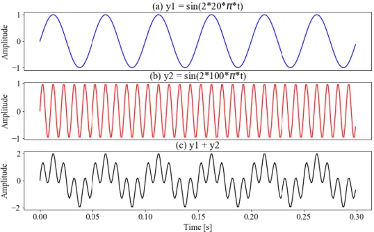
Since the frequency of coma and brain-death EEG was lower than 40Hz, 80 sets of

standard artificial signals were selected to test the computational performance of 3

static EMD-based algorithms. Each of standard artificial signals was composed of a

low frequency sinusoidal signal of each different frequency and the high frequency

sinusoidal signal of 100 Hz, in which the frequency range of the low frequency

sinusoid signals was 0∼40Hz and the interval frequency was 0.5Hz. Take a simple

example shown in figure. 2.1.

Fig. 2.1 Standard artificial signals. (a) was the low frequency sinusoidal signal of 20Hz, (b)

was the high frequency sinusoidal signal of 100 Hz, (c) was the standard artificial signals composed by (a) and (b).

2.1.2 Coma and Brain-Death EEG

The EEG data we used in the paper were recorded in EEG preliminary examination

(25)

11

families [27]. During the EEG recording, patient was lying on the bed in the ICU. And

the EEG data was detected by the portable NEUROSCAN ESI-64 system and a laptop

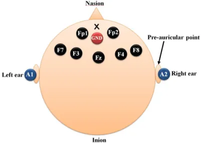
computer. Six exploring electrodes (Fp1, Fp2, F3, F4, F7, F8) as well as one ground

electrode (GND) were placed on the forehead, and two reference electrodes (A1, A2)

were placed on earlobes. And the sampling frequency was 1000Hz and the electrode

resistance was lower than 8KΩ. The placement of electrodes was shown in figure. 2.2. In this paper, the EEG of 35 coma and quasi-brain-death patients (male:21; female:14)

with a total of 36 cases of EEG (coma:19; quasi-brain-death:17), in which there were

one case of EEG in coma and one case of EEG in quasi-brain-death included in the

same special patient whose state was from coma state in the first EEG recording

process to quasi-brain-death state in the second EEG recording process after about 10

hours.

Fig. 2.2 The placement of 9 electrodes.

2.2 Energy Feature Extraction Methods

2.2.1 Static EMD-Based Algorithms

Static EMD-based algorithms, EMD, MEMD and 2T-EMD are fully data-driven

algorithms for multiscale decomposition and time-frequency analysis of real-valued

(26)

12

non-linear and non-stationary signal is decomposed into a finite set of IMFs (Intrinsic

Mode Functions) and a monotonic residual signal based on local time feature scale of

signal. As shown in figure 2.3. Here the IMF must satisfy two conditions, one is the

number of zero crossing and the number of extrema differing at most by one, and the

other is that the upper and lower envelopes of the signal are symmetrical.

As described in formula (2-1), for a real-valued signal 𝑥(𝑡), the algorithm principle of EMD is to decompose 𝑥(𝑡) into a finite set of IMFs ∑𝑛=𝑁_𝑛=1 𝐼𝑀𝐹_𝑛 and a monotonic residual signal 𝑟(𝑡).

𝑥(𝑡) = ∑𝑛=𝑁_𝑛=1 𝐼𝑀𝐹_𝑛+ 𝑟(𝑡) (2-1)

Fig. 2.3 Basic Schematic of static EMD-based algorithms.

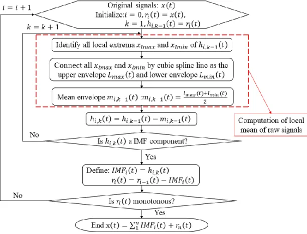
The principle flow chart of EMD is shown in figure 2.4. The key of EMD

algorithm is the computation of local mean of the original signal, which is computed

by taking the average of upper envelopes and lower envelopes. The envelope is

obtained by connecting all local extrema through using cubic spline line. Specifically,

for a single channel signal 𝑥(𝑡), extract all local maximum 𝑥𝑙𝑚𝑎𝑥 and all local

minimum 𝑥_𝑙_𝑚𝑖𝑛, and connect all 𝑥_𝑙_𝑚𝑎𝑥 and 𝑥_𝑙_𝑚𝑖𝑛 by using cubic spline line respectively to get the upper envelope 𝐿𝑚𝑎𝑥(𝑡) and lower envelope 𝐿𝑚𝑖𝑛(𝑡). Then

(27)

13

Fig. 2.4 The principle flow chart of EMD.

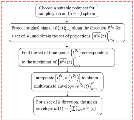
But for multivariate signals, the local extrema may not be defined directly. The

MEMD algorithm solved this problem by taking signal projections along different

directions in n-dimensional spaces, and these signal projections are then averaged to

obtain the local mean. More specifically, for a multivariate signal with n components

{𝑣⃗(𝑡)}_𝑡=1𝑇 _{= {𝑣}

1(𝑡), 𝑣2(𝑡), ⋯ 𝑣𝑛(𝑡)}𝑡=1𝑇 which is a sequence of n-dimensional

vectors, and a set of direction vectors {𝑥⃗𝜃𝑘_}

𝑘=1 𝐾

= {𝑥𝜃1_{, 𝑥}𝜃2_{, ⋯ , 𝑥}𝜃𝐾_{} that are along}

the directions given by angels {𝜃⃗_𝑘}

𝑘=1 𝐾

= {𝜃₁, 𝜃₂, ⋯ 𝜃_𝐾} on a (𝑛 − 1) sphere, the computation of local mean of MEMD algorithm is shown in figure 2.5 [29].

Although the MEMD algorithm can be used to decompose multivariate signals,

with using real-valued projections along multiple directions on hyperspheres in order

to calculate the local mean of the multivariate signals, which may result in a large

(28)

14

Fig. 2.5 Flow chart of the computation of local mean for MEMD.

The 2T-EMD offers the possibility to decompose multi-channel signals without

projections by redefining and computing the signal mean envelope, and the

re-definition of the signal mean trend, which is obtained by interpolating between

barycenter of particular oscillation, or called elementary oscillation. Specifically, the

key of 2T-EMD is the computation of signal mean trend, which is obtained by

averaging two envelopes: a first envelope interpolates the even indexed barycenters

which include signal borders, and a second envelope interpolates the odd indexed

barycenters which also include signal borders [30]. Moreover, the 2T-EMD can

process single and multi-channel signals. Let s be a class 𝐶1_{function in} _𝑅𝐷

domain and differentiable with a continuous first derivative. The sifting procedure of

computing the signal mean trend is briefly illustrated as Algorithm (1) [31]. And the

(29)

15

Algorithm 1 2T-EMD Algorithm

1. Defined a time series 𝑇⃗⃗(𝑠) as the tangent vector to s and express as: 𝑇⃗⃗(𝑠): 𝑡 → [1,𝑑𝑠

𝑑𝑡(𝑡)]

2. Defined 𝛼_𝑠 as the Euclidean inner products of 𝑅𝐷+1_{and express as:}

𝛼𝑠: 𝑡 → 𝑙𝑖𝑚 ℎ→0〈𝑇

⃗⃗_𝑠_{(𝑡 − ℎ), 𝑇}⃗⃗_𝑠_{(𝑡 + ℎ)〉}

Due to the continuity of Euclidean inner product, so αs can be expressed as:

∀𝑡 ∈ 𝑅, 𝛼_𝑠(𝑡) = 𝑙𝑖𝑚

ℎ→0〈𝑇⃗⃗𝑠(𝑡 − ℎ), 𝑇⃗⃗𝑠(𝑡 + ℎ)〉

3. Since s is a class 𝐶1_{function, we can get the formula below:}

∀𝑡 ∈ 𝑅, 𝛼_𝑠(𝑡) = ‖𝑇⃗⃗_𝑠(𝑡)‖2 = 1 + ‖𝑑𝑠 𝑑𝑡(𝑡)‖

2

Where ‖∙‖ refers to the Euclidean norm of both 𝑅𝐷 and 𝑅𝐷+1. 4. Oscillation extremum of function 𝑠(𝑡) is defined as below:

𝛽_𝑠(𝑡): 𝑡 → 𝛽_𝑠(𝑡) = ‖𝑑𝑠 𝑑𝑡(𝑡)‖

2

5. Take two consecutive oscillation extrema, respectively 𝑃₁ = [𝑡₁, 𝑠(𝑡₁)] 𝑇_and

𝑃₂ = [𝑡₂, 𝑠(𝑡₂)] 𝑇_{, thereby} _𝑀

𝑃1−𝑃2, the barycenter of the associated elementary

oscillation is defined as below:

𝑀𝑃1−𝑃2 = [ 𝑡₁ + 𝑡₂ 2 , 1 𝑡1− 𝑡2 ∫ 𝑠(𝑡)𝑑𝑡 𝑡1 𝑡2 ] 𝑇

6. The mean vector 𝑒⃗(𝑡) of signal can be obtained according to the definition. In conclusion, there are two aspects of principle differences among EMD, MEMD,

and 2T-EMD, respectively the number of channels analyzed and the computation

method of local mean of original signals. The comparison of EMD, MEMD, and

(30)

16

Fig. 2.6 Flow chart of the computation of local mean for 2T-EMD.

Table 2-1 Algorithm Principle Comparison among EMD, MEMD, and 2T-EMD

Method Similarity

Differences

Type of signal Computation method of local mean EMD _Original signal 𝒔(𝒕) ∑ 𝑰𝑴𝑭𝒊 𝒏 𝒊=𝟏 + 𝒓(𝐭) (𝒓(𝒕) is residual) Single channel

The local mean is calculated as the half sum of the upper and the lower envelopes, obtained by interpolating between local minima and maxima using cubic splines.

MEMD Multi-channel

Take signal projections along different directions in n-dimensional spaces, and averaged corresponding projections to obtain the local mean.

2T-EMD Single channel

and multi-channel

(31)

17

2.2.2 Dynamic 2T-EMD

In order to observe dynamic changes of EEG energy and reduce the influence by

noise, Dynamic 2T-EMD is developed by extending 2T-EMD with excellent static

EEG energy computational performance. As is shown in figure 2.7, a time window

that the width is ∆𝑡 and a time step with the width ∆𝜆 are introduced in the Dynamic 2T-EMD algorithm, where ∆𝑡 and ∆𝜆 are controllable parameters. With the time window sliding along the time axis in a time step, a time step of EEG is

processed and value is stored. Then steps above are repeated to get the dynamic EEG

energy features [32].

Fig. 2.7 Schematic diagram of Dynamic 2T-EMD

(32)

18

Algorithm 2 Dynamic 2T-EMD Algorithm

1. Initialize the number of iteration 𝑗 = 1, the number of IMF 𝑖 = 1,, and the number of time step 𝑘 = 0; and set 𝑟⃗_𝑖(𝑘 ∙ ∆𝑡) = {𝑠⃗(𝑘 ∙ ∆𝑡)}_𝑘=0𝐾 _,_ℎ_⃗⃗

𝑖,𝑗−1(𝑘 ∙ ∆𝑡) =

𝑟⃗𝑖(𝑘 ∙ ∆𝑡).

2. Compute the barycenter 𝑀_{(𝑖,𝑗−1)}

𝑃𝑘𝑥−𝑃𝑘𝑥+1(𝑘 ∙ ∆𝑡) of random consecutive

oscillation extrema 𝑃_𝑘_𝑥 and 𝑃_𝑘_𝑥+1 in the period of 𝑘 ∙ ∆𝑡 , that is 𝑀_{(𝑖,𝑗−1)} 𝑃𝑘𝑥−𝑃𝑘𝑥+1(𝑘 ∙ ∆𝑡) = [ 𝑘𝑥∙∆𝑡+𝑘𝑥+1∙∆𝑡 2 , 1 𝑘𝑥∙∆𝑡−𝑘𝑥+1∙∆𝑡∫ ℎ ⃗⃗_{𝑖,𝑗−1}_{(𝑡)𝑑𝑡} 𝑘𝑥∙∆𝑡 𝑘𝑥+1∙∆𝑡 ] 𝑇 .

3. Obtain the signal mean trend 𝑒⃗𝑖,𝑗−1(𝑘 ∙ ∆𝑡) by interpolating between oscillation

barycenters of ℎ⃗⃗_{𝑖,𝑗−1}(𝑘 ∙ ∆𝑡).

4. Subtract e⃗⃗_i,j−1(k ∙ ∆t) from the given signals ℎ⃗⃗𝑖,𝑗−1(𝑘 ∙ ∆𝑡) , we define

ℎ⃗⃗𝑖,𝑗(𝑘 ∙ ∆𝑡) = ℎ⃗⃗𝑖,𝑗−1(𝑘 ∙ ∆𝑡) − 𝑒⃗𝑖,𝑗−1(𝑘 ∙ ∆𝑡). If ℎ⃗⃗𝑖,𝑗(𝑘 ∙ ∆𝑡) obey the sifting stop

criteria, define 𝐼𝑀𝐹⃗⃗⃗⃗⃗⃗⃗⃗⃗_𝑖(𝑘 ∙ ∆𝑡) = ℎ⃗⃗_𝑖,𝑗(𝑘 ∙ ∆𝑡), otherwise repeat the iteration steps from (2) to (4). It is worth noting that the stop criteria is using the Cauchy-like

criteria, more precisely, let 𝑑_𝑖,𝑗 be the 𝑖 − 𝑡ℎ IMF computed at the 𝑗 − 𝑡ℎ iteration of the sifting process, then the sifting criteria is for instance 90% of

values ‖𝑑𝑖,𝑗+1(𝑡)−𝑑𝑖,𝑗(𝑡)

𝑑𝑖,𝑗(𝑡) ‖ are lower than 10-2.

5. Define 𝑟⃗_𝑖(𝑘 ∙ ∆𝑡) = 𝑟⃗_𝑖(𝑘 ∙ ∆𝑡) − 𝐼𝑀𝐹⃗⃗⃗⃗⃗⃗⃗⃗⃗_𝑖(𝑘 ∙ ∆𝑡), if the result signal is monotonous, we can get the decomposition results of signals during 𝑘 ∙ ∆𝑡, that is 𝑠⃗(𝑘 ∙ ∆𝑡) = ∑𝑁 𝐼𝑀𝐹⃗⃗⃗⃗⃗⃗⃗⃗⃗_𝑖(𝑘 ∙ ∆𝑡) + 𝑟⃗_𝑁(𝑘 ∙ ∆𝑡)

𝑖=1 , otherwise repeat steps from (2) to (5).

6. Determine whether the elapsed time 𝑘 ∙ ∆𝑡 exceeds the end time 𝑇2, if it does,

the process goes to end and the final decomposition result {𝑠⃗(𝑘 ∙ ∆𝑡)}_𝑘=0𝐾 = {∑𝑁 𝐼𝑀𝐹⃗⃗⃗⃗⃗⃗⃗⃗⃗_𝑖(𝑘 ∙ ∆𝑡) + 𝑟⃗_𝑁(𝑘 ∙ ∆𝑡)

𝑖=1 }_𝑘=0

𝐾

; If it doesn't, moving the time window and

(33)

19

2.3 Results

2.3.1 Results of Comparison among 3 Static EMD-Based Algorithms

In this section, EMD, MEMD and 2T-EMD were compared from experimental

aspect based on standard artificial signals and coma and brain-death patients’ EEG

respectively, in which signal representation accuracy and computational time were

compared for standard artificial signals as well as computational time was compared

based on coma and brain-death patients’ EEG. Here signal representation accuracy

was denoted by root-mean-square error (RMSE), shown as formula (2-2). RMSE was

used to measure the deviation of processed value and original value, where N is

sampling frequency, 𝑥𝑖 is the amplitude of artificial signals after processing by

algorithms, 𝑜_𝑖 is the amplitude of original standard artificial signals. RMSE = √1

𝑁∑ (𝑥𝑖− 𝑜𝑖) 2 𝑁

𝑖=1 (2-2)

A. Results Based on Standard Artificial Signals

The first part is that EMD, MEMD and 2T-EMD were compared based on standard

artificial signals. From the content explained in section 2.2.1, we know that EMD

algorithm and MEMD algorithm can only be used to process single channel signals

and multi-channel signals respectively, while 2T-EMD can process both single and

multi-channel signals. So comparison between EMD and 2T-EMD based on single

channel standard artificial signals, and comparison between MEMD and 2T-EMD

(34)

20

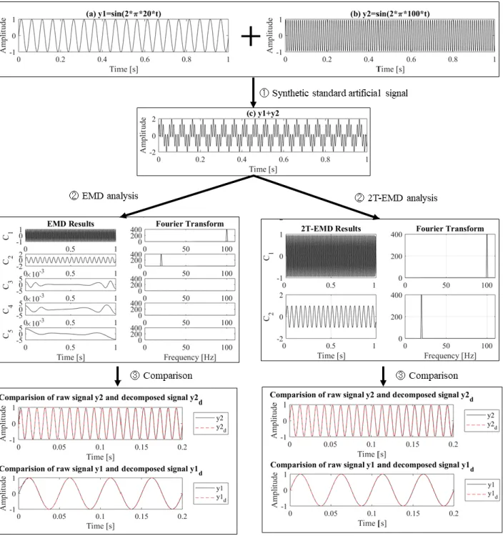
Fig. 2.8 Analysis process of EMD and 2T-EMD based on single channel standard artificial

signals. The upper panel ① was the synthesis process of two sinusoid signals 𝑦1 = 𝑠𝑖𝑛 (2 ∗ 𝜋 ∗ 20 ∗ 𝑡) and 𝑦2 = 𝑠𝑖𝑛 (2 ∗ 𝜋 ∗ 100 ∗ 𝑡); the middle panel ② was the decomposition process of EMD, 2T-EMD and their corresponding Fourier Transform process; the lower panel ③ was the comparison of raw signals and decomposed signals.

(35)

21

signals explained in section 2.1.1. As shown in figure 2.8 was a simple example to

explain intuitively the analysis process of EMD and 2T-EMD based on standard

artificial signals.

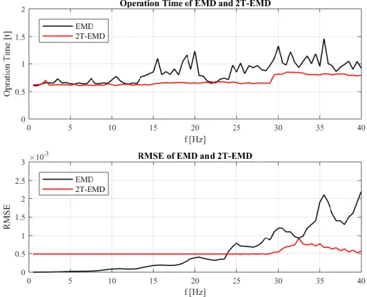
Fig. 2.9 Comparison of operation time and RMSE for EMD and 2T-EMD based on single

channel standard artificial signals.

As is shown in the upper panel of figure 2.9, the computational time of 2T-EMD is

less than 1s and remains the stable duration range of 0.6s ~ 0.85s, while the computational time of EMD fluctuates greatly in the range of 0.6s ~ 1.6s, and is longer than that of 2T-EMD, even reach twice of 2T-EMD. It takes different

computation time to decompose signals of different frequencies for EMD algorithm,

while it almost takes the same computation time for 2T-EMD. And as is shown in the

(36)

22

has better integrated performance in both computational time and the signal

representation accuracy based on single channel standard artificial signals.

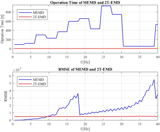
Fig. 2.10 Comparison of operation time and RMSE for MEMD and 2T-EMD based on

multi-channels standard artificial signals.

Secondly, computational time and RMSE of MEMD and 2T-EMD based on

multi-channel standard artificial signals were compared. In this comparison, the

number of multi-channel was set to 6, and the 80 synthetic artificial standard signals

mentioned in section 2.1.1 were divided into 13 groups, with 6 channels per group

from low to high frequency.

B. Results Based on Coma and Brain-Death Patients’ EEG

In the second part, the computational time of EMD, MEMD and 2T-EMD based on

patients' EEG explained in section 2.1.2 were compared. And it was also divided into

two aspects, where one is comparison between EMD and 2T-EMD based on patients'

(37)

23

on patients' EEG of multi-channel.

Firstly, EMD and 2T-EMD are used to analyze 36 cases of patients’ EEG data for

random single channel. As is shown in figure 2.11, the computational time of

2T-EMD algorithm is 1.5s ~2.0s, slightly shorter than that of EMD algorithm, which is in the range of 1.9s ~6.8s. So it takes shorter time to process single channel EEG for 2T-EMD compared with EMD.

Fig. 2.11 Comparison of operation time for EMD and 2T-EMD based on 36 cases of coma

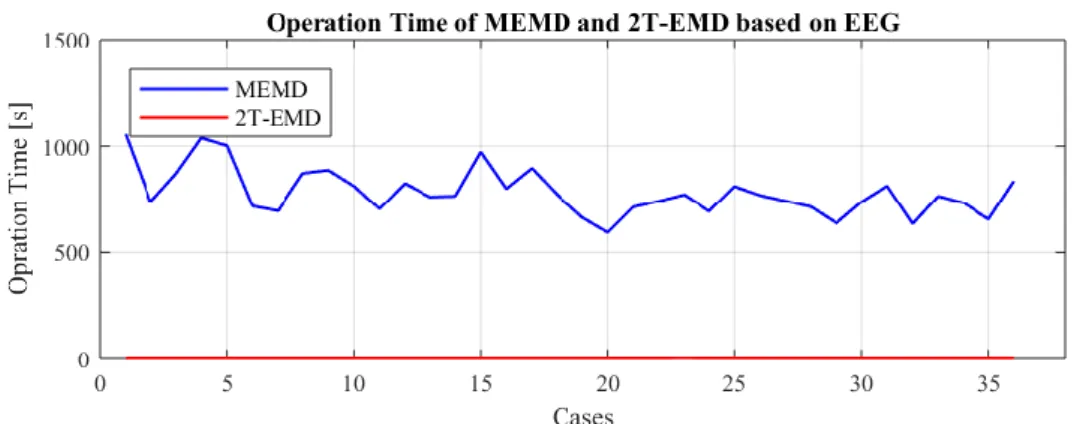
Fig. 2.12 Comparison of operation time for MEMD and 2T-EMD based on 36 cases of coma

Secondly, MEMD and 2T-EMD were used to decompose the 36 cases of coma and

brain-death patients' EEG data for 6 channels. As is shown in figure 2.12, the

(38)

24

2T-EMD algorithm works much faster than MEMD algorithm for multi-channel EEG.

In summary, it is obvious that the optimal computational performance of 2T-EMD

is the best among EMD, MEMD, 2T-EMD for both single and multi-channel signals

[33].

2.3.2 Results of Dynamic 2T-EMD Based on Patients’ EEG

In this section, the EEG of 35 coma and brain-death patients (male: 21; female: 14)

with a total of 36 cases of EEG (coma: 19; quasi-brain-death: 17) were processed by

Dynamic 2T-EMD and descriptive statistics measure, in order to obtain the

differences of EEG energy between coma patients and brain-death patients.

Specifically, it was explained from overall and individual aspects. Firstly, in order to

give an overall dynamic EEG energy distribution results for coma group and

brain-death group, 60s EEG data were randomly selected from every of 36 cases of

coma and brain-death EEG, and analyzed by Dynamic 2T-EMD and descriptive

statistics measure. Secondly, from individual point of view, two typical cases of EEG

from two different patients who were in coma and brain-death state respectively, and

one special patient whose EEG was from coma state to brain-death state were

processed by Dynamic 2T-EMD.

A. Results for 36 Cases of Coma and Brain-Death Patients’ EEG

Since coma and brain-death patients’ EEG data were recorded in the ICU, which

were mixed with complex noise, statistical analysis visual analysis were used to

analyze the energy data processed by Dynamic 2T-EMD to improve the accuracy and

reliability of results. In this paper, we focused on visual descriptive statistical analysis

method. Descriptive statistics are summary statistics that quantitatively describe or

summarize features of a collection of information [34]. Here basic measures of

(39)

25

were applied to evaluate dynamic energy data obtained, in which mean and median

were used to describe the central tendency of data set, and standard deviation and

percentile were introduced to evaluate the dispersion of data set.

Descriptive statistical analysis was conducted to EEG energy features processed by

Dynamic 2T-EMD. Specifically, since duration of every case of EEG was different,

60s EEG data were selected from 19 cases of EEG in coma state and 17 cases of EEG

in brain-death state to process by using Dynamic 2T-EMD algorithm to extract EEG

energy features firstly. And EEG energy features obtained were grouped from three

aspects, which were different cases, different channels, and different states

respectively. And then the EEG energy features grouped were evaluated by applying

descriptive statistical analysis.

There were 4 steps to conduct the experiment measure:

(1) Select randomly 60s EEG data from 36 cases of coma and quasi-brain-death

patients’ EEG (coma: 19; quasi-brain-death: 17). Here there were 5 channels of EEG data with values equal 0 from 3 cases of EEG invalid.

(2) Process these EEG data by applying Dynamic 2T-EMD algorithm and 211

time-energy series (36 cases × 6 channels - 5 invalid series) were obtained.

(3) Group the 211 time-series according to 3 ways:

① Divide the 211 time-series into 36 groups according to 36 cases.

② Divide the 211 time-series into 12 groups according to 2 states and 6 channels. ③ Divide them into 2 groups according to 2 states.

(4) Analyze time-energy series after grouping by using descriptive statistical analysis,

in which the mean and median were computed to evaluate the central tendency and

(40)

26

Fig. 2.13 The statistical analysis results of EEG energy for 36 coma and quasi-brain-death

EEG for average channel.

a. Static Statistical Results for 36 Cases of Patients’ EEG

In this part, 211 time-energy series were grouped into 36 set of data based on cases.

The mean, median, standard deviation and quantile were computed for every case for

(41)

27

and median of EEG energy for coma case is higher than that for brain-death case for

average channel. Here the mean and median energy fluctuation range of coma cases

are 1.10 × 104 ~ 6.66 × 104 and 1.01 × 104 ~ 6.22 × 104, which are higher than 1.00 × 104_{, while the mean and median energy fluctuation range of brain-death cases}

are 2.48 × 103 ~ 9.13 × 103 and 2.40 × 103 ~ 8.86 × 103, which are no lower than 1.00 × 104_{. Moreover, it is also shown that the variance range of standard}

deviation of coma cases is wider than that for brain-death cases from figure 2.13(b)

and figure 2.13(c).

b. Static Statistical Results Based on 2 States – 6 Channels

Fig. 2.14 The statistical analysis results of EEG energy for coma group and quasi-brain-death

group at each channel.

In order to get characteristics of EEG energy for coma group and brain-death group

in different channels of this batch of EEG energy data, 211 time-energy series were

grouped into 12 set of data based on 2 states and 6 channels. Mean, median, standard

deviation and quantile were also calculated for the 12 set of data. As shown in figure

2.14(a), (b) and (c), it is obviously observed that the mean and median of coma group

is higher than that of brain-death group for every channel, and the range of energy

change of every channel for coma group is wider than that for brain-death group.

(42)

28

value of every channel for 2 groups were shown in Table 2-2 and table 2-3, in which

percent is defined as 𝑝𝑒𝑟𝑐𝑒𝑛𝑡 =(𝑀𝑒𝑎𝑛−𝑀𝑒𝑑𝑖𝑎𝑛)

𝑀𝑒𝑎𝑛 , it is used to measure the difference

between mean and median value. In general, it is shown that the percent for

brain-death group is lower compared with the percent for coma group.

Table 2-2 Mean, median and percent of EEG energy for coma group at every channel.

Coma Channel Fp1 Fp2 F3 F4 F7 F8 Mean 31946 32951 31666 28708 23772 23804 Median 23735 24299 26274 24351 17303 18872 Percent 25.7% 26.3% 17.0% 15.18% 27.2% 20.7%

Table 2-3 Mean, median and percent of EEG energy for brain-death group at every channel Brain- death Channel Fp1 Fp2 F3 F4 F7 F8 Mean 3899 4147 4410 4756 4201 4962 Median 3461 3734 3581 3787 3521 4564 Percent 11.23% 9.96% 18.80% 20.37% 16.19% 8.02%

Here the characteristics of energy for coma group and brain-death group for

average channel were shown in figure 2.15, in which there were 114 time–energy

series (19 cases × 6 channels - 5 invalid series) for coma group and 102 time-energy

series (17 cases × 6 channels) for brain-death group. As can be seen from figure 2.15

(a) and figure 2.15 (b), the distribution of energy data for coma group is intuitively

higher than that for brain-death group, in which the mean of both group are

2.88 × 104_and _{4.40 × 10}3_{, and the median of both group are} _{2.24 × 10}4_and

(43)

29

c. Static Statistical Results Based on 2 States – Average Channel

Fig. 2.15 The error bar and box plot of coma group and brain-death group for average

channel.

d. Dynamic Statistical Results Based on 2 States – Average Channel

In this part, 19 cases of EEG data for coma group and 17 cases of EEG data for

brain-death group were analyzed by Dynamic 2T-EMD. Here the time window of

Dynamic 2T-EMD was set to 1s and no overlap among time windows. Then we took

mean value, 5 quantile values (5%, 25%, 50%, 75%, and 95%) of every second for

channels averaged for coma group and brain-death group respectively due to the two

groups were not balanced. As shown in figure 2.16, it is obviously observed that the

dynamic EEG energy distribution of channels averaged for coma group is higher than

that for brain-death group.

(44)

30

averaged channels. Coma group is marked in black and brain-death group is marked in red. Thick lines show median line of data. Thick dashed lines show mean line of data. Dark filled bands highlight 25%-75% of data. Light filled bands highlight 5%-95% of data.

And as shown in figure 2.17, we also analyzed the dynamic EEG energy

distribution for every channel (Fp1, Fp2, F3, F4, F7 and F8) for both coma group and

brain-death group. It is shown there exists significant differences of EEG energy

distribution among different channels for coma group and brain-death group.

Fig. 2.17 Dynamic EEG energy distribution of coma group and brain-death group for 6

channels.

A. Results for 2 Typical Cases and 1 Special Case of Patients’ EEG a. Results for 2 Typical Cases of Coma and Brain-Death Patients’ EEG

(45)

31

In this part, we selected 60s EEG data from the coma patient's EEG with recording

time of 937s as well as 60s EEG data from the brain-death patient's EEG with

recording duration of 905s. As is shown in figure 2.18, it is intuitively observed the

dynamic change of EEG energy for the two typical cases. The range of dynamic EEG

energy of the coma patient's EEG is 3.5 × 104 ~ 1.1 × 105, while it's 1.8 × 103_{~ 4.1 × 10}3_{for the brain-death patient's EEG.}

a. Results for 1 Special Cases of Patient’s EEG from Coma State to Brain-Death State

Moreover, the special patient's EEG whose state was from coma to brain-death state

was processed, in which 60s EEG data from coma EEG segment and 60s EEG data

from brain-death segment were selected to analyzed by Dynamic 2T-EMD. As is

shown in figure 2.18, for the same patient, the EEG energy distribution for coma state

is higher than that for brain-death state, which is consistent with that for coma group

and brain-death group. And the distribution range of EEG energy for the special

patient' EEG decreases from 1.7 × 104 ~ 4.1 × 104 to 2.4 × 103 ~ 5.8 × 103 [35].

Fig. 2.18 Dynamic EEG energy distribution of average channel for the patient who was from

coma state to brain-death state.

2.4 Chapter Summary

In this chapter, three static EMD-based EEG energy extracted algorithms (EMD,

(46)

32

from algorithm principle and experiments, where experiments based on both standard

artificial signals and quasi-brain-death patients’ EEG respectively. Hereafter, the

Dynamic 2T-EMD algorithm is firstly proposed by dynamically extending 2T-EMD.

Then 36 cases of coma and brain-death patients’ EEG were analyzed by the proposed

algorithm. Moreover, two typical patients’ EEG who were in coma state and in

brain-death state respectively, as well as one special patient’s EEG who was from

coma state to brain-death state were also analyzed by Dynamic 2T-EMD from

individual perspective. EEG energy features obtained then analyzed by descriptive

statistical measure. Final results illustrated that there was a significant differences of

(47)

33

Chapter 3 Epilepsy EEG Analysis

3.1 Materials

Fig. 3.1 EEG time series of Bonn dataset

The epilepsy EEG dataset used in this paper is from the Department of

Epileptology at the University of Bonn [36]. The dataset is public available and used

widely in the research of epilepsy EEG data analysis and classification. There were 5

sets in the dataset, denoted as set A, set B, set C, set D and set E. Each of set

contained 100 single-channel EEG segments with recording duration of 23.6s per

segment. The sampling rate and band-pass filter were set 173.61Hz and 0.53∼40Hz. In

details, set A and set B were surface EEG recordings taken from five healthy

volunteers who were relaxed in an awake state with eyes open (A set) and eyes closed

(B set). Set C, set D and set E were intracranial EEG recordings originated from five

patients, in which set C and set D were taken from during seizure free intervals from

(48)

34

D), set E were taken from epileptic seizure activity. In this part, C set, D set and E set

were studied. As shown in figure 3.1 is the EEG time series of C set, D set and E set

for Bonn dataset.

3.2 Methodology

3.2.1 Phase-Amplitude Coupling

Fig. 3.2 The process of filtering and Hilbert Transform. (a) was the single-channel time series

𝑥⃗(𝑛) (𝑛 = 1, … , 𝑁) . (b) and (c) were the low-frequency oscillation 𝑥⃗⃗⃗ (𝑛) and 𝑙

high-frequency oscillation 𝑥⃗⃗⃗⃗ (𝑛) filtered by band-pass filter, where the range of ℎ

low-frequency and high-frequency were set to 4Hz – 8Hz and 30Hz – 40Hz. (d) and (e) were low-frequency phase time series ∅⃗⃗⃗ (𝑛) and high-frequency amplitude time series 𝑎𝑙 ⃗⃗⃗⃗ (𝑛) ℎ

computed by Hilbert Transform.

Phase-amplitude coupling is explained as that the high-frequency amplitude is

(49)

35

high-frequency amplitude time series were computed firstly before evaluating the

phase-amplitude coupling strength. In this paper, band-pass filtering and Hilbert

Transform were used, in which FIR (finite impulse response) filters was applied to

filter. Take an example, for a single-channel time series 𝑥⃗(𝑛) (𝑛 = 1, … , 𝑁) , band-pass filtered was applied to extracted high-frequency oscillation interested

𝑥_ℎ

⃗⃗⃗⃗ (𝑛) and low-frequency oscillation interested 𝑥⃗⃗⃗ (𝑛). Then Hilbert Transform was _𝑙 used to extract corresponding instantaneous phase and instantaneous amplitude of

both oscillations. As shown in formula (3-1), we got two analytic signals.

𝑧_𝑙 ⃗⃗⃗ (𝑛) = 𝑎⃗⃗⃗ (𝑛)𝑒_𝑙 𝑖∅⃗⃗⃗⃗ (𝑛)𝑙 _, _𝑎 𝑙 ⃗⃗⃗ (𝑛) = |𝑧⃗⃗⃗ (𝑛)| _𝑙 𝑧_ℎ ⃗⃗⃗⃗ (𝑛) = 𝑎⃗⃗⃗⃗ (𝑛)𝑒_ℎ 𝑖∅⃗⃗⃗⃗⃗ (𝑛)ℎ _{, 𝑎} ℎ ⃗⃗⃗⃗ (𝑛) = |𝑧⃗⃗⃗⃗ (𝑛)| (3-1) _ℎ Where ∅⃗⃗⃗ (𝑛) and ∅𝑙 ⃗⃗⃗⃗ (𝑛) were the instantaneous phase time series, as well as ℎ

𝑎_𝑙

⃗⃗⃗ (𝑛) and 𝑎⃗⃗⃗⃗ (𝑛) were the instantaneous amplitude time series of both _ℎ high-frequency oscillation and low-frequency oscillation. It is shown in figure 3.2 that

the process of band-pass filtering and Hilbert Transform before computing coupling

strength.

A. Modulation Index (MI) of Phase-Amplitude Coupling

There are five methods to quantify the phase-amplitude coupling strength also

called MI. The first method was proposed by Canolty et.al, which evaluated

phase-amplitude coupling strength by computing the normalized MI [37]. The

algorithm is illustrated as Algorithm (3).

Algorithm 3 Phase-amplitude coupling algorithm proposed by Canolty

1. Defined a complex variable, where ah is the amplitude time series of high

frequency oscillation, ∅⃗⃗⃗ is the phase time series of low frequency oscillation: _𝑙

(50)

36

2. Compute the absolute value of the mean vector based on 𝑧 (𝑛) and defined the result as ‘MI’: 𝑀_𝑟𝑎𝑤 = |1 𝑁∑ 𝑍 (𝑛) 𝑁 𝑛=1 |

3. Using surrogate data approach to compute the surrogate 𝑧⃗⃗⃗ (𝑛) (𝑛 = 1, … , 𝑁; 𝑠 =_𝑠 1, … , 𝑆) by introducing an arbitrary time lag between ∅⃗⃗⃗ and 𝑎_𝑙 ⃗⃗⃗⃗ . And compute the _ℎ mean vector 𝑀𝑠 = |

1

𝑁∑ 𝑧⃗⃗⃗ (𝑛)𝑠 𝑁

𝑛=1 | of 𝑧⃗⃗⃗ (𝑛) as step 2. 𝑠

4. Repeat the step 3 for 𝑠 = 1, … , 𝑆 times to obtain the surrogate values 𝑀₁, … , 𝑀_𝑆, and compute the mean 𝜇 and standard variance 𝜎 of these surrogate values.

5. Compute the normalized modulation index which is denoted as 𝑀:

𝑀 =𝑀𝑟𝑎𝑤− 𝜇 𝜎

The second method to quantify the phase-amplitude coupling is the PLV

(phase-locking value) method [38-40]. The algorithm is illustrated as Algorithm (4).

Algorithm 4 The Phase-amplitude coupling algorithm based on PLV

1. Apply secondly Hilbert Transform to 𝑎⃗⃗⃗⃗ , and get the analytic signal of 𝑎ℎ ⃗⃗⃗⃗ as ℎ

below:

𝑍_𝑎_ℎ

⃗⃗⃗⃗⃗⃗ = 𝑎⃗⃗⃗⃗⃗⃗ (𝑛)𝑒_𝑎_ℎ 𝑖∅⃗⃗⃗⃗⃗⃗⃗⃗ (𝑛)𝑎ℎ _{(𝑛 = 1, … , 𝑁)}

Where 𝑎⃗⃗⃗⃗⃗⃗ (𝑛) and ∅𝑎ℎ ⃗⃗⃗⃗⃗⃗ (𝑛) are the amplitude time series and phase time series of 𝑎ℎ

𝑎ℎ

⃗⃗⃗⃗ (𝑛).

(51)

37 𝑃𝐿𝑉 = |1 𝑁∑ 𝑒 𝑖(∅⃗⃗⃗⃗ (𝑛)−∅𝑙 ⃗⃗⃗⃗⃗⃗⃗⃗ (𝑛))_𝑎ℎ 𝑁 𝑛=1 |

Where the PLV value is used to measure the coupling strength.

The third method to measure the phase-amplitude coupling was based on GLM

(general linear model) [41]. The algorithm is explained in Algorithm (5).

Algorithm 5 The Phase-amplitude coupling algorithm based on GLM

1. Create a new high-frequency amplitude model by introducing a multiple regression

as below and compute the residual vector 𝑒 . 𝑎_ℎ ⃗⃗⃗⃗ = 𝑋 𝛽 + 𝑒 Where 𝑋 = [𝑐𝑜𝑠 (∅⃗⃗⃗ (𝑛)) 𝑠𝑖𝑛 (∅𝑙 ⃗⃗⃗ (𝑛))𝑙 1 ⋮ 1 ] 𝑁×3 (𝑛 = 1, … 𝑁) , 𝛽⃗⃗⃗ are regression

coefficients by using Least-Squares solution, 𝑐𝑜𝑠 (∅⃗⃗⃗ (𝑛)) and 𝑠𝑖𝑛 (∅𝑙 ⃗⃗⃗ (𝑛)) are the 𝑙

cosine and sine transform of low-frequency phase time series respectively.

2. Compute the value described as the model:

𝑟_𝐺𝐿𝑀2 = 𝑆𝑆(𝑎⃗⃗⃗⃗ ) − 𝑆𝑆(𝑒 )ℎ 𝑆𝑆(𝑎⃗⃗⃗⃗ )_ℎ

Where 𝑆𝑆(𝐴_ℎ) and 𝑆𝑆(𝑒) are the sum of squares of high-frequency amplitude time series 𝑎⃗⃗⃗⃗ and the sum of squares of error 𝑒 . The 𝑟_ℎ _𝐺𝐿𝑀2 is used to quantify the coupling strength.

The fourth method to measure the phase-amplitude coupling was based on an

adaptive of the KL distance (Kullback-Leibler distance) [42]. The algorithm is

explained in Algorithm (6).

(52)

38

1. Construct the composite time series [∅⃗⃗⃗ (𝑡) 𝑎_𝑙 ⃗⃗⃗⃗ (𝑡)], which present the amplitude _ℎ of low-frequency oscillation at each corresponding phase of the low-frequency

rhythm.

2. Divide the phases ∅⃗⃗⃗ (𝑡) into bins in order, and compute the mean value of 𝑎_𝑙 ⃗⃗⃗⃗ (𝑡) _ℎ in each phase bin 𝑗, where the mean value is expressed by ⟨𝑎_ℎ⟩_∅_𝑙(𝑗).

3. Normalize the mean value ⟨𝑎_ℎ⟩_∅_𝑙(𝑗): 𝑃(𝑗) = ⟨𝑎𝑓𝐴⟩_∅ 𝑓𝑃(𝑗) ∑ ⟨𝑎𝑓𝐴⟩_∅ 𝑓𝑃(𝑗) 𝑁_𝑏𝑖𝑛𝑠 𝑗=1

Where N_bins is the number of phase bins.

4. There is no coupling between high-frequency amplitude and low-frequency phase

if the mean value ⟨𝑎_ℎ⟩_∅_𝑙(𝑗) at each phase bin is the same, namely the phase-amplitude distribution 𝑃 is consistent with uniform distribution 𝑈 ; if different, there is coupling. So a new MI is defined to measure the difference of

phase-amplitude distribution and uniform distribution by adapting KL distance. The

new MI is described as:

𝑀𝐼 = 𝐷𝐾𝐿(𝑃, 𝑈) 𝑙𝑜𝑔 (𝑁_𝑏𝑖𝑛𝑠)

Where 𝐷_𝐾𝐿(𝑃, 𝑈) = 𝑙𝑜𝑔(𝑁_𝑏𝑖𝑛𝑠) − 𝐻(𝑃), 𝐻(𝑃) = − ∑𝑁_𝑏𝑖𝑛𝑠_𝑗=1 𝑃(𝑗)𝑙𝑜𝑔 [𝑃(𝑗)].

The fifth method to quantify the phase-amplitude coupling strength was proposed

by Ozkurt. et.al. [43]. The value to quantify the phase-amplitude coupling strength 𝜌 is defined as below: 𝜌 = 1 √𝑁 |∑𝑁𝑛=1𝑎ℎ(𝑛)𝑒𝑖∅𝑙(𝑛)| √∑𝑁𝑛=1𝑎ℎ(𝑛)2 (𝑛 = 1, … , 𝑁) (3-2) B. Phase-Amplitude Comodulogram

Phase amplitude comodulogram is the graphical representation that exhibits

(53)

39

over a grid of frequencies. When there is no priori assumption of frequency bands

phase-modulating and the amplitude-modulated, the comodulogram can be used to

locate initially the frequency bands which coupling occurs. As shown in figure 3.3,

the frequency of phase 𝑓_𝑃 is represented in the horizontal axis and the frequency of amplitude 𝑓𝐴 is displayed in the ordinate axis. The phase-coupling strength at the

band [𝑓𝐴(𝑖) 𝑓𝑃(𝑗)] is denoted using a pseudocolor plot with hot color indicating

high coupling strength.

Fig. 3.3 The example of comodulogram.

3.2.2 Support Vector Machine (SVM)

SVM is a supervised learning method based on statistical learning theory (SLT) in

machine learning. The basic model is the linear classifier that defines the largest

interval in the feature space. It maps the vector to the high-dimensional feature space

through nonlinear mapping, and then selects the most classified surface to obtain a

hyperplane segmentation, which can separate the two types of modes and ensure the

interval is maximized. It is suitable for solving classification problems with low

sample size in high-dimensional complex nonlinear systems. For example, as shown

in figure 3.4, for a linear classification in two dimensional plane, there is a binary

201901繆堯 学位博士論文 (4.06MB)