Multivariate EEG feature analysis and its
application on brain death determination
and brain computer interface
by
Gaochao Cui
EEG
EEG
EEG Brain death determination, BDD
Brain computer interface, BCI BDD EEG [1][2] EEG EMD EMD EMD MEMD [3] MEMD EEG Dynamic-MEMD
Dynamic-MEMD MEMD EEG
EEG MEMD Dynamic-MEMD EEG EEG BDD ApEn [4] EEG EEG permutation entropy, PE EEG PE
alpha theta delta
Dynamic-MEMD PE
partial
[5]
BCI EEG
EEG BCI
(MI) BCI P300 BCI
EEG PDC
3 Dynamic-MEMD PE PDC
EEG EEG
Abstract
Electroencephalography (EEG) is a recording of voltage fluctuations resulting from ionic current flows within the neurons of the brain and refers to the recording of the brain’s spontaneous electrical activity over a short period of time. It is widely used in clinical diagnosis of brain diseases and brain research. The objective of this dissertation is to use different feature analysis methods to process the EEG signal. The main works include the EEG-based analysis on brain death determination (BDD) and brain computer interface (BCI).
Brain death is defined as the irreversible loss of all functions of the brain, including the brainstem. In clinics, death of brain therefore qualifies as death, as the brain is essential for integrating critical functions of the body. Notably, a reliable, safe and rapid method in the determination of brain death, the EEG-based preliminary examination has been proposed in [1][2] by our laboratory. In my dissertation, three kinds of feature analysis methods are performed including energy, complexity and connectivity feature analysis.
For energy feature analysis, an adaptive algorithm for MEMD called dynamic MEMD (Dynamic-MEMD) are proposed to calculate and evaluate the EEG energy. In the mentioned preliminary examination, the empirical mode decomposition (EMD) method is used to decompose a single-channel recorded EEG data into a number of components with different frequencies. From there, the components which are related to the brain activities were selected to compute EEG energy using power spectrum analysis technique for evaluating the differences between comatose patients and quasi-brain-deaths. Moreover, multivariate empirical mode decomposition (MEMD) method, an extensions approach of EMD, also proposed in [3] to calculate and evaluate the EEG energy in which the main advantage is to extract brain activity features from multi-channel EEG simultaneously. However, by using MEMD, it is difficult to observe EEG energy variation for subjects. While by using Dynamic-MEMD, we can not only denoise the original EEG data but also calculate the EEG energy of subjects in a dynamic duration. From the result, we distinguish three consciousness levels of heathy people in rest state, patients in comatose and brain death. The results show the effectiveness of the proposed method in differentiating for consciousness levels, which can be applied into the development of real-time BBD system further.
which is different from energy feature analysis in frequency domain. Two different complexity parameters are used including dynamic approximate entropy (ApEn) and permutation entropy (PE). Dynamic ApEn measures crossing all channels along the time-coordinate of EEG signal to observe the variation of the dynamic complexity which can be used to monitor the state changing online [4]. Compared with other complexity parameters, PE has the better performance in clinic EEG analysis offline [5]. Results show that ApEn and PE can distinguish from heath people, comatose patients and brain death along time coordinate and in different bands respectively. For connectivity analysis, the time-varying information flow between channels are calculated based on partial directed coherence (PDC), which combined the time and frequency domain. Energy and complexity analysis are focusing on the property of single channel while connectivity analysis can find out relationship between channels. Result show that the connectivity of coma patients is much stronger than brain death, but weaker than health subjects.
On the other side, through appropriate external stimuli like visual and auditory, some EEG feature components can be evoked (called evoked potentials). Brain computer interface system is to control external devices based on EEG evoked potentials. Based on different kinds of external stimuli, there are many kinds of BCI system, such as motor image (IM) based BCI, steady-state visual evoked potentials (SSVEP) based BCI and P300-based BCI [6][7][8]. P300-based brain computer interface (BCI), often called P300 speller, is one of the most successful paradigm, which has shown advantages in terms of high accuracy and short training time. However, the existing P300-based BCI employs single type of external stimuli, such as visual stimuli, which limits their performance in clinical applications.
In this dissertation, an eight-class hybrid-BCI system based on multiple modalities of P300 evoked by simultaneous audio and visual stimuli is proposed. The experimental results show the significant difference in event related potential (ERP) between single type and multiple types of stimuli. The experiment results demonstrate the effectiveness of our new BCI paradigm, which outperforms the visual or audio P300 in terms of higher accuracy and information transfer rates (ITR). Hybrid-BCI has extensive potential in high performance and stability BCI system development.
. Chapter 1 describes the background and objective of EEG-based BDD and BCI system. This chapter describes the definition of brain death, and the brain dead determine the flow. The significance of brain-dead judgment research and the importance of brain-dead judgment system are also introduced. In addition, the definition of BCI system and the type of BCI system are introduced.
. Chapter 2 describes methods of data analysis for brain death determination. Based on these basic methods, it is difficult to observe EEG energy variation of subjects. To solve this problem, an adaptive algorithm was proposed to calculate and evaluate the energy of EEG recorded from the healthy subjects, comatose patients and brain deaths and observe the state changes of patients’ consciousness. Moreover, to study the connectivity between each channel, granger causality analysis and graph theory are also introduced in this chapter.
Chapter 3 describes the analysis results based on the mentioned methods in chapter 2. By using dynamic-MEMD, EEG energy can be calculated in time series for subjects. In addition, EEG energy variation of subjects could increase the reliability and show three groups of healthy subjects in rest state, comatose patients and brain death. The analyzed results show the effectiveness and performance of the proposed method in calculation of EEG energy for evaluating consciousness levels.
Chapter 4 describes the data processing methods that are used to build BCI system. Furthermore, tensor factorization method for incomplete EEG data are also descripted in this chapter. For incomplete EEG signals, tensor factorization method can be used to complete the missing data of EEG signal.
Chapter 5 describes a hybrid-BCI system with visual and audio stimuli that proposed in this dissertation. The experimental results show the significant difference in ERPs between visual stimuli and multiple types of stimuli. The classification accuracy results demonstrate the effectiveness of our BCI paradigm, which outperforms the visual P300. On the other hand, a fully Bayesian CP factorization for incomplete tensors method is used to analysis real EEG data. Experimental results show that, this method has a better performance on incomplete EEG signal with certain degree of data missing ratio. Classification results also proved the availability of this method. But if the data missing ratio of EEG signal was very high, this method will recover EEG data not very well.
In BDD research, by using dynamic-MEMD which is proposed in this dissertation, EEG energy of subjects can be calculated in a dynamic duration. From the result, three consciousness levels of heathy people in rest state, patients in comatose and brain death can be distinguished. By using PE feature analysis method, the brain death and comatose can be distinguished in different bands of EEG signal. From the analysis result of PDC method, the connectivity of coma patients is much stronger than brain death, but weaker than health subjects.
In BCI research, higher accuracy and information transfer rates (ITR) can be obtain based on this hybrid-BCI system. It has extensive potential in high performance and stability BCI system development.
CONTENTS
Chapter 1 Introduction………..………….………..…………...…….1
1.1 Brain death determination (BDD)………..…….…………..1
1.2 Brain computer interface (BCI)……...….3
1.3 Chapter summary………...5
Chapter 2 Method of feature analysis for brain death determination…..……...6
2.1 Energy feature analysis………..………6
2.1.1 Empirical mode decomposition (EMD) algorithm………….…..…...6
2.1.2 Multivariate empirical mode decomposition (MEMD) algorithm…..8
2.1.3 Dynamic MEMD (D-MEMD) algorithm……….….…………10
2.2 Complexity feature analysis………..……….10
2.2.1 Approximate Entropy (ApEn) algorithm………..……..….…..…10
2.2.2 Multi-scale permutation entropy algorithm……….……..…12
2.3 Connectivity feature analysis………...…..13
2.3.1 Brain network construction based on PDC….………....…13
2.4 Chapter summary……….…………..15
Chapter 3 Analysis results of brain death determination………….….……..….16
3.1 Energy feature analysis results.………..………..16
3.1.1 Analysis result based on EMD algorithm………….……..…..……16
3.1.2 Analysis result based on MEMD algorithm………....…..……19
3.1.3 Analysis result based on D-MEMD algorithm………...……..….…21
3.2 Complexity feature analysis results.………25
3.2.1 Analysis result based on ApEn algorithm………..…….………...25
3.2.2 Analysis result based on Multi-scale PE algorithm…………..……28
3.3 Connectivity feature analysis results………...………29
3.3.1 Analysis result of brain network construction based on PDC……..29
Chapter 4 Method of data analysis for brain computer interface………34
4.1 Support vector machine (SVM) algorithm………...…..…..34
4.2 Linear discriminant analysis (LDA) algorithm………..….…..…...35
4.3 Tensor factorization for incomplete EEG data algorithm………..…..…35
4.4 Chapter summary……….37
Chapter 5 Hybrid brain computer interface system…………...………….….…38
5.1 Subjects………...38
5.2 Experimental stimuli and paradigm……….…………..……..……38
5.2.1 P300 experiment based on visual stimuli………...…….…40
5.2.2 P300 experiment based on audio stimuli……….……….…40
5.2.3 P300 experiment based on hybrid stimuli……….…………40
5.3 EEG data acquisition and processing………….………...….41
5.4 Feature extraction and classification………....…..……..41
5.5 Information transfer evaluation………..…….…..……..42
5.6 Results of classification and information transfer evaluation………...…42
5.7 EEG signal completion based on tensor factorization…….………….…45
5.8 Chapter summary……….48
Chapter 6 Conclusions……….……...………..…...……...49
6.1 Conclusion of BDD………...…..49
6.2 Conclusion of BCI……….………..49
6.3 Future works of BDD and BCI………49
6.4 Chapter summary……….50
Chapter 1 Introduction
1.1 Brain death determination (BDD)
Brain death is defined as the irreversible loss of all functions of the brain, including the brainstem. The three essential findings in brain death are coma, absence of brainstem reflexes and apnea [9]- [10]. In clinics, death of brain therefore qualifies as death, as the brain is essential for integrating critical functions of the body. The equivalence of brain death with death is largely, although not universally, accepted [9]. The diagnosis of brain death is very important. Guidelines for determining brain have been proposed for example the apnea test and brainstem function detection [10]. Notably, it is commonly accepted that EEG might serve as an auxiliary and useful tool in the confirmatory tests, for both adults and children [11]- [14].
EEG has been effectively used into diagnosis diseases in clinics and related research area [15]- [17]. It has several nice features forwarding the applications in clinical practice and science research. Non-invasion feature makes it easily accessible and safe to be used in used. Specifically, patients in the deep coma state could be recorded the frontal area of head without big operations, decreasing the risks resulted from movement. High time resolution (milliseconds) feature enables it to catch the real-time dynamic changes of neural activity. Simple and friendly operation steps feature motivate wide-use of EEG in both theory and practice area such as disease diagnosis and classification. EEG can record continuous signals where is much safer than the test on patients’ spontaneous breathing with unplugging the ventilator intermittently. Even though there are such several strong points in EEG application for brain death detection, the reasons for improvement of EEG analysis on brain death diagnosis should be paid attention to are summarized as follows.
among which the error rate of parameter setting was the highest (11.40%), followed by those of result determination (10.44%), recording techniques (10.25%), environmental requirements (7.46%) and pitfalls (3.68%). We can see that the doctors with professional knowledge of medicine would make mistakes of operations on EEG even if during the period of training program. In the clinic, the accuracy and in time diagnosis of disease for patients in coma is so urgent that the improvement of interpretation of clinical EEG is so necessary and needs to be highly emphasized.
(2). Distinguish from coma and brain death should be confirmed. Patients in coma may or may not progress to brain death and they often show symptoms of absence of movement, and breathing occasionally less brainstem activity, whose clinic performance is like brain death. But what is the difference inner mechanism and how come we don’t consider a coma to be temporary brain death. We should understand the point in definition of brain death, irreversible loss of functions of the brain, while coma is temporary loss of conscious but still alive [19]-[20].
preliminary examination system as a reliable yet safety and rapid way for the determination of brain death [2]. That is, after above items 1)- 3) have been verified, and an EEG preliminary examination along with real-time recorded data analysis method is applied to detect the brain wave activity at the bedside of patient. On the condition of positive examined result, we suggest to stop the brain death diagnosis process and spend more time on the medical care.
In this thesis, EMD, MEMD, ApEn and other methods are used to analysis the clinical EEG signal of brain death, coma patients and health subjects. Based on these research, a dynamic MEMD method is proposed, which analyzes the signals over a period of time. Furthermore, Granger causality analysis and graph theory are used to analysis the EEG signal of clinical and constructed the brain network. It is used to analysis the correlation between channels during different brain activity status.
1.2 Brain computer interface (BCI)
Brain computer interface (BCI) is a new type of human interface that can contribute to the augmentation of human capabilities, namely for people affected by severe motor disabilities. BCI system can directly translates the EEG signals into control signals that people can use them to control external devices without using their nerves and limbs [23]. Recently, there has been a great process in research and development of brain-controlled devices based on BCI system [24]- [26]. For instance, users can essential to operate a relatively sophisticated device, such as a computer mouse, a wheelchair, a prosthetic limb, a robot, etc. [27]- [33]. Furthermore, the research on BCI applied to human control of physical devices has been broadly focused mainly in two directions: neuroprosthetics and brain-actuated wheelchairs [34]. Neuroprosthetics focuses on the motion control or hand orthosis, which usually improves the upper body possibilities of users with mobility impairments, such as reachability and grasping. Wheelchairs focus on the facilitation of assistance in mobility to accomplish complex navigational tasks to improve quality of life and self-independence of users [35] [36].
system: invasive BCI and noninvasive BCI. For invasive BCI, EEG recording electrodes are placed on the cerebral cortex in surgically [42]. Using invasive BCI, people can obtain high quality and complex control signals and a high speed of information transfer. However, the subjects need to take the risk of brain surgery and long-term viability with chronic invasive neural probes [43]. For noninvasive BCIs, subjects could avoid the risk of surgery and simplify experimental procedures. Currently, the brain signals for noninvasive BCIs include functional magnetic resonance imaging (fMRI), magnetoencephalography (MEG), functional near infrared spectroscopy (fNIRS) and Electroencephalography (EEG). Among them, EEG has been widely used in BCI system because of its convenience. Although EEG-based BCI also have good real-time response, technically less demanding and a lower cost, but its low signal-noise ratio (SNR) and low spatial resolution limit the performance of EEG-based BCI system. In clinical application, many neurological diseases such as amyotrophic lateral sclerosis (ALS) and some certain types of cerebral palsy where there is no control of voluntary movements. A number of studies report that individuals with ALS can have impaired eye movements and slowing of saccades [37].
by mind and physical activity. The stimulus can be visual, audio, somatosensory, etc. [42][43]. In previous studies, most of the ERP P300-based BCI system generally used single type sense organ to accept external stimuli, such as audio, visual, tactile sensation and so on [44]-[45]. The single pathway of receiving stimulation, is one reason of low information transfer rates (ITR). It also can make people feel irritable and fatigue when people accept same kind of stimuli for a long time. In this situation, the participants will easily to be influenced by ambient noise and affect the BCI system performance. In this thesis, we attempt to take advantage of audio and visual simultaneously in EEG-based hybrid BCI system. It means that when a user receives visual stimuli, will also receive an auditory stimulus. In our experiments, we did three different situations of tests under the same experimental conditions: P300 based visual stimuli, audio stimuli and hybrid stimuli. And then, the results based on three different situations tests will be compared and analyzed. Our experiments proved that this experimental method can indeed improve the performance of BCI system.
1.3 Chapter summary
Chapter 2. Data analysis methods for brain death determination
2.1 Energy feature analysis
2.1.1 Empirical mode decomposition (EMD) algorithm
The EMD method for analyzing nonlinear and nonstationary data was proposed in Huang et al. (1998). This method is used to decompose the data into several oscillatory components called intrinsic mode function (IMF). The IMF components are usually expressed as the standard Hilbert transforms, from which the instantaneous frequencies can be calculated. The local energy and the instantaneous frequency derived from the IMF components through the Hilbert transform can be given a full energy-frequency-time distribution of the data.
For an observed time-domain signal !(#), we can always obtain its Hilbert transform %(#), such as %(#) =1 () * !(+) # − + - .-/+. (2 − 1) It is impossible to calculate the Hilbert transform as an ordinary improper integral because of the pole at + = #. However, the ) in front of the integral denotes the Cauchy principal value which expands the class of functions for the integral in Equation (2-1).
With this definition, !(#) and %(#) form the complex conjugate pair, so the complex signal 3(#) can be formulated as
3(#) = !(#) + 5%(#) = 6(#)789(:) (2 − 2)
where j is the imaginary unit (5; = −1), an instantaneous amplitude 6(#) and an
instantaneous phase <(#) are presented by
6(#) = =!;(#) + %;(#) (2 − 3)
<(#) = #6?.@A%(#)
!(#)B (2 − 4) The instantaneous frequency D(#) of the signal !(#) can be defined as
D(#) = /<(#)
In principle, it is necessary that one limitation is a narrow band signal for the instantaneous frequency by Equation (2 −5).
An IMF component as a narrow band signal is a function that satisfies two conditions: (1) In the whole data set, the number of extrema and the number of zero crossings must be either equal or differ at most by one.
(2) At any point, the mean value of the upper envelope with the lower envelope is zero. Here the upper envelope is defined by the local maxima, and the lower envelope is defined by the local minima.
The procedure to obtain the IMF components from an observed signal is called sifting and it consists of the following steps:
(1) Identification of the extrema of an observed signal.
(2) Generation of the waveform envelopes by connecting local maxima as the upper envelope, and connection of local minima as the lower envelope.
(3) Computation of the local mean by averaging the upper and lower envelopes. (4) Subtraction of the mean from the data for a primitive value of IMF component. (5) Repetition of the above steps, until the first IMF component is obtained.
(6) Designation of the first IMF component from the data, so that the residue component is obtained.
(7) Repetition of the above steps, the obtained residue component contains
information about longer periods which will be further resifted to find additional IMF components.
The sifting algorithm is applied to calculate the IMF components based on a criterion by limiting the size of the standard deviation (SD) computed from the two consecutive sifting results as FG = H IJℎL.@(#) − ℎL(#)M ; ℎL.@; (#) N (2 − 6) P :QR
!(#) = H ST(#) + UV(#) (2 − 7)
V TQ@
where ST(#), (Y = 1, … , ?) represents ? IMF components, and UV represents a residual component which can be either the mean trend or a constant.
2.1.2 Multivariate empirical mode decomposition (MEMD) algorithm
For multivariate signals, the local maxima and minima may not be defined directly because the fields of complex numbers and quaternions are not ordered. Moreover, the notion of ‘oscillatory modes’ defining an IMF is rather confusing for multivariate signals. To deal with these problems, the multiple real-valued projections of the signal is proposed. The extrema of such projected signals are then interpolated component wise to yield the desired multidimensional envelopes of the signal. In MEMD, we choose a suitable set of direction vectors in n-dimensional spaces by using: (i) uniform angular coordinates and (ii) low-discrepancy pointiest.
The problem of finding a suitable set of direction vectors that the calculation of the local mean in an n-dimensional space depends on can be treated as that of finding a uniform sampling scheme on an n sphere. For the generation of a point set on an (? − 1) sphere, consider the ? sphere with center point [ and radius \, given by
\ = HJ!8− [8M; (2 − 8)
V^@ 8Q@
A coordinate system in an n-dimensional Euclidean space can then be defined to serve as a pointset on an (? − 1) sphere. Let {<@, <; ,· · ·, <V.@ } be the (? − 1)
angular coordinates, then an ?-dimensional coordinate system having {!T}TQ@V as the
? coordinates on a unit (? − 1) sphere is given by
involves the family of Halton and Hammersley sequences. Let !@, !; ,· · ·, !V be the
first ? prime numbers, then the Yth sample of a one-dimensional Halton sequence, denoted by UTh is given by UTh = 6R ! + 6@ ! ; +6; ! i + ⋯ +6j ! j^@ (2 − 10) where base-! representation of Y is given by
Y = 6R + 6@× ! + 6;× !;+ ⋯ + 6
j× !j (2 − 11)
Starting from Y = 0, the Yth sample of the Halton sequence then becomes JUThl, U
Thm, UThn, ⋯ , UT
hoM (2 − 12)
Consider a sequence of ? -dimensional vectors {p(#)}:Q@P = {q
@(#), q;(#),· · ·
, qV(#)} which represents a multivariate signal with ? -components, and r9s =
{!@L , !
;L ,· · · , !VL } denoting a set of direction vectors along the directions given by
angles <L = {<@L , <
;L ,· · · , <V.@L } on an (? − 1) sphere. Then, the proposed
multivariate extension of EMD suitable for operating on general nonlinear and non-stationary ?-variate time series is summarized in the following.
(1) Choose a suitable point set for sampling on an (? − 1) sphere. (2) Calculate a projection, denoted by tu9s(#)v
:Q@ P
, of the input signal {p(#)}:Q@P
along the direction vector r9s , for all k (the whole set of direction vectors),
giving tu9s(#)v LQ@ w
as the set of projections.
(3) Find the time instants {#T9s} corresponding to the maxima of the set of projected
signals tu9s(#)v LQ@ w . (4) Interpolate [#T9s, py# T
9sz] to obtain multivariate envelope curves t79s(#)v LQ@ w
. (5) For a set of K direction vectors, the mean |(#) of the envelope curves is
to !(#) − /(#), otherwise apply it to /(#).
The stoppage criterion for multivariate IMFs is similar to the standard one in EMD, which requires IMFs to be designed in such a way that the number of extrema and the zero crossings differ at most by one for F consecutive iterations of the sifting algorithm. The optimal empirical value of S has been observed to be in the range of 2-3. In the MEMD, we apply this criterion to all projections of the input signal and stop the sifting process once the stopping condition is met for all projections.
2.1.3 Dynamic-MEMD algorithm
The Dynamic-MEMD is an adaptive algorithm of the MEMD. We have defined the EEG energy using the power spectrum within the frequency band multiplied by recorded EEG time. To observe EEG energy variation of subjects, we extend MEMD in the temporal domain along time-coordinate of EEG signal. Supposing a multivariate EEG data series p(#) consisting of ~ segments (epochs) {pV(#)}VQ@ , the MEMD can
be carried out through each segment.
The Dynamic-MEMD is defined as the MEMD applied to all segments such that p(#) = [p@(#), … , p(#)] = ÄH SL,@(#) + U@(#), … , H SL,V(#) + U(#) wÅ LQ@ wl LQ@ Ç (2 − 14) where p(#) are residue signals and {SL,V(#)}LQ@wo are IMF components with
}V (? = 1, … , ~) being the number of IMFs for the segmented nth signal p(#). Consequently, in our experiment, we remove the residue signal \(#) and 3 IMFs
from {SL,V(#)}LQ@wo which is not expected, and combine the (N − Q) IMFs to be the
denoised signal. We have defined the EEG energy using the power spectrum within the frequency band multiplied by recorded EEG time. Thus, we change the denoised signal from time domain to frequency domain by Fast Fourier Transformation and integrate it to compute the EEG energy.
2.2 Complexity feature analysis
ApEn is a regularity statistic quantifying the unpredictability of fluctuations in a time series that appears to have potential application to a wide variety of physiological and clinical time-series data [12], [13]. Intuitively, one may reason that the presence of repetitive patterns of fluctuation in a time series renders it more predictable than a time series in which such patterns are absent.
Given a time series {!(?)}, (? = 1, … , ~), to compute the ÉuÑ?(!(?), |, U) (|: length of the series of vectors, U: tolerance parameter) of the sequence, the series of vectors of length | , q(Ö) = [!(Ö), !(Ö + 1), … , !(Ö + | − 1)] is firstly constructed from the signal samples {!(?)}. Let G(Y, 5) denote the distance between two vectors q(Y) and q(5) (Y, 5 ≤ ~ − | + 1), which is defined as the maximum difference in the scalar components of q(Y) and q(5), or
G(Y, 5) = max
äQ@,…,ã|qä(Y) − qä(5)| (2 − 15)
Then, we further compute the ~ã,ç(Y), which represents the total number of vectors
q(5) whose distance with respect to the generic vector q(Y) is less than U , or G(Y, 5) ≤ U. Now define [ã,ç(Y), the probability to find a vector that differs from q(Y)
less than the distance U. And éã,ç, the natural logarithmic average over all the vectors
of the [ã,ç(Y) probability as
[ã,ç(Y) = ~ã,ç(Y)
~ − | + 1 (2 − 16) éã,ç(Y) =∑.ã^@TQ@ êëí[ã,ç(Y)
~ − | + 1 (2 − 17) For | + 1, repeat above steps and compute éã^@,ç. ApEn statistic is given by
ÉuÑ?(!(?), |, U) = éã,ç− éã^@,ç (2 − 18)
The typical values | = 2 and r between 10% and 25% of the standard deviation of the time series {!(?)} are often used in practice [12].
signal as
ÉuÑ?(F, |, U) = ÉuÑ?(!@(?), |, U), … , ÉuÑ?(!(?), |, U) (2 − 19) Consequently, in our experiment, the ÉuÑ?(F(?), |, U) statistic measures the
variation the of complexity of a EEG data series F. The occurrence of irregular pattern of one interval is excepted to be followed by the next in brain-death EEG.
2.2.2 Multi-scale permutation entropy algorithm
Permutation entropy is a complexity parameter method based on comparison between adjacent values of time series whose performance is similar to other chaotic dynamical systems such as Lyapunov exponent. Unlike some other non-linear monotonic transformation methods, its features include simple, easier to calcite and stronger anti-jamming capability [23]. Multi-scale permutation entropy is a measurement method of finite length time series complexity. Compared with the traditional entropy method with fixed scale factor, multi-scale permutation entropy creates a coarse-grained continuous time series through the coarse graining transformation. And then calculate the data using entropy which fulfil the changing from the single static entropy value to the dynamics entropy sequence [24]. The key functions are from formula 2-20 to 2-22.
Coarse-grained processing is got by formula 2-20, permutation probability 2-21 and entropy 2-22. Here, the length of original EEG data is ì. î is expressed for scale factor, | is the embedding dimension. ~ corresponds to the number of m! permutation cases on the constructed sequence.
2.3 Connectivity feature analysis
2.3.1 Brain network construction based on PDC
Partial directed coherence (PDC) is proposed to express Granger Causality in a new way based on MVAR (multivariate autoregressive) model. Normalized PDChû→h† accounts for the proportion between xT flowing to x8 and signals outgoing from x8. PDChû→h† is nearer 0 and then it means no much connection while its value is greater than 0.1, which is regarded as the two channels connected to each other [11]. Specifically, the algorithm will be discussed below [12-13]. A time-varying N-variate AR process of order p could be expressed in formula 2-23.
⎣ ⎢ ⎢ ⎢ ⎢ ⎡rr@ ; . . . rL⎦⎥ ⎥ ⎥ ⎥ ⎤ = H Éç ⎣ ⎢ ⎢ ⎢ ⎢ ⎡!!@(? − Y) ;(? − Y) . . . !L(? − Y)⎦⎥ ⎥ ⎥ ⎥ ⎤ + ⎣ ⎢ ⎢ ⎢ ⎢ ⎡ßß@(#) ;(#) . . . ßL(#)⎦⎥ ⎥ ⎥ ⎥ ⎤ ñ TQ@ (2 − 23)
where µ is the noise vector and ∑ñTQ@Éç is given by formula 2-24. Éç(?) = I
6@@ç ⋯ 6@Lç
⋮ ⋱ ⋮
6L@ç ⋯ 6LLç
N (2 − 24) Here, we process the brain death EEG data of 6 channels k = 6 so first the AR model of EEG in time domain should be solved. And then do the FFT on formula 2. The time-varying version of partial directed coherence is defined as formula 2-25,
PDChû→h†(%) = ÉT,8(%) ™68´(%)68(%)
(2 − 25)
where 68(%) is the 5#ℎ column of the matrix É(%). PDChû→h†(%) is normalized where the higher value (taking 0.3 as the border) in a certain frequency band represents the linear influence from channel Y to channel 5. As a result, we will get a connectivity matrix (6 multiple 6) to test the information flow strength and direction between two channels in EEG data.
map, we can analyze the characteristics for coma and brain death groups and then to locate the abnormal connectivity in brain death.
In the graph, the connectivity between channels is illustrated by connectivity matrix. We have 6 nodes in the network so the size of adjacency matrix is 6 6. Suppose the adjacency matrix is B and ¨T8 is the element of B. If ¨T8 = 1 and then there is connection between node Y and 5. Else ¨T8 = 0 and then there is no connection from node Y to 5 . So, the constructed brain network based on PDC value is directed weighted network. But some of the parameters of network would be transferred into two-value one to be analyzed and calculated. We use three topological graph parameters to do quantificational estimation.
1) Degree: for our network graph, degree has in-degree and out-degree respectively. In-degree represents the number of edges importing into the certain node; out-In-degree shows the number of edges out of the node. The value degree could be used as the evaluation of the node importance level in the network.
2) Clustering coefficient: the clustering degree could be measured by clustering coefficient, showing the probability of the connectivity between each node adjacency edge. The formula 2-26 and 2-28 is taken as the calculated function for node Y and the average whole network.
ìT =
2Së??7S#7/7T
ÖT(ÖT− 1) (2 − 26) ì =∑T∈ÆìT
~ (2 − 27) 3) Betweenness centrality: the role and importance could be described by betweenness centrality. The value of it is bigger, the more important of the node in the network (named core node). The solved function is formula 2-28. The Ø8L means the number of optimal path from node 5 to node Ö.
In this thesis, the specific steps for brain network construction of these two groups data based on PDC value are given as follows. There are 10 adult patients’ EEG data for the two groups. Each patient has a corresponding PDC matrix 6 6. Set different threshold values ω0(ωmin ≤ ω0 ≤ ωmax) for PDC, where ωmin = 0.1 and ωmax = 1.79. The single sampling t-test is applied to determine every group functional connectivity and then the final brain network structure will be fixed.
Suppose the sample mean value is D≥ and the zero hypothesis is given as follows: ¥R: D ≤ DR, ¥@: D > DR
The test statistic function is given in formula 2-29. # =D≥ − DR
™î; ?
(2 − 29)
If # is in the reject domain and then the connectivity strength between each channel is bigger than DR, which means that there is connection between the corresponding nodes
in the brain network; else there is no connection. 2.4 Chapter summary
Chapter 3. Analysis results of brain death determination
3.1 Energy feature analysis
3.1.1 Analysis result based on EMD method
The first case is concerned with an 18-year-old male patient (Patient A). The patient had a primary cerebral disease and was admitted to the hospital in April 2004. After one month of hospitalization, the patient lost consciousness and went into a deep-coma state. His pupil dilated to 2 mm, and a respiratory machine was used. In June, the patient presented symptoms similar to that of a brain-death case. On the same day, the EEG examination was taken for 710s.
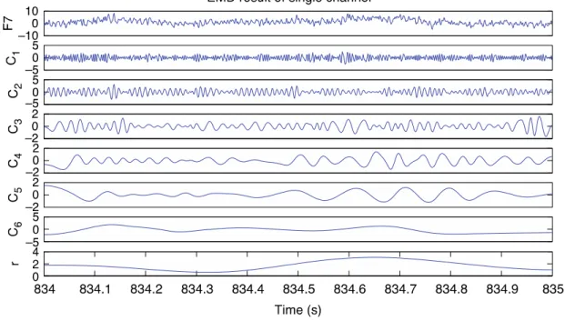
From the EEG signal, we paid close attention to a raw EEG signal of a randomly chosen channel in one second. For instance, the signal of channel F4 in the time range 217-218 s is selected as an example. By applying the EMD method described in Section 2 to the chosen signal, as shown in Fig. 3-1, we obtained five IMF components (C1– C5) and a residual component (r). In this case, the high-frequency component (C1) and the residual component (r) are not the typical useful components considered.
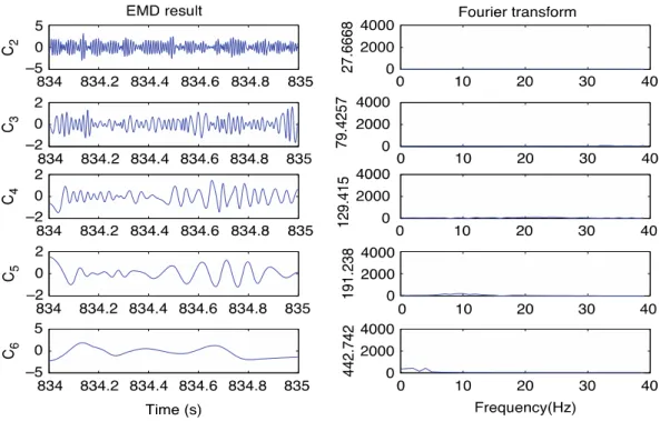
Then, the remaining four IMF components (C2–C5), as desirable ones, are displayed in the frequency domain by applying the fast Fourier transform (FFT). As shown in Fig. 3-2, the right column gives the peak value of each IMF component’s power spectra in their frequency domain. With y-coordinate in the scope from zero to 4000, one component with a frequency of 12 Hz was visualized (the third block in right column of Fig. 3-2. This component corresponds to the range of alpha wave that we mentioned before. Compared to other components, its peak value of power goes up to 2578.69 that reflects a high intensity of brain activity. The patient was in a coma state but the analysis result indicated the patient still had physiological brain activity. With the aid of further therapy, this patient regained consciousness.
components shown in Fig. 3-3.
Fig. 3-1 EMD result of single channel
Fig. 3-2 EMD result and its Fourier transform
noted in distinguishing the results of the above two cases. The y-coordinate of Fig. 3-4 is in the same scope as the one of Fig. 3-2 from 0 to 4000, however, the amplitudes of IMF components this time are all in a low range. The maximum value of IMFs’ in the power spectra is only 422.742.
It is clear that by comparing the frequency amplitude plots for Patients A and B, the brain activity of Patient B within the range up to 13 Hz is significantly weaker. Thus, the brain activity could hardly be seized except for the irregular noise. Without loss of generality, the same process was applied to other channels and time points. Only similar results could be obtained. Further clinical diagnosis of this case concluded that the patented had been in the brain-death state.
Fig. 3-4 EMD result and its Fourier transform 3.1.2 Analysis result based on MEMD method
In this part, we use MEMD to analysis the coma patients’ EEG signal. Through the MEMD method described, we obtained 9 IMF components (C1 to C9) with different frequency from high to low. Each IMF carries a single frequency mode, illustrating the alignment of common scales within different channels. Therefore, generally in our experiment, the IMF components from C1 to C3 with the same high frequency scales refer to electrical interference or other noise from environment that contains in the recorded EEG. The residual component (r) is not the typical useful components considered, either. The desired components from C4 to C9 are combined to form the denoised EEG signal, and changed into frequency domain by fast Fourier transform (FFT). As showed in Fig. 3-5, the upper line gives each channels denoised EEG signal in time domain, and the lower line display the denoised EEG signal of each channel in their frequency domain. With y-coordinate in the scope from 0 to 7000 in the frequency domain, we find the value of power spectra at 2-10 Hz is very high. The average energy of each channel is 2.14×10⁴. The analysis result indicated the patient still had strong
Furthermore, clinical diagnosis from the doctor confirm the patient is in a coma state at recorded time.
Fig.3-5 MEMD result of coma patient
Then we use the MEMD to analysis the brain death patient’s EEG. As showed in Fig. 3-6, with the same analysis of the first patient, contrary to the first patient power spectrum, the value is in a low range. The average energy of each channel is 0.229×10⁴.
The analysis result indicate that this patient physiological brain activity is extremely low and we suspect the patient was in the quasi-brain- death state. Later, the clinical doctor confirms this result is correct.
0 0.5 1 −500 50 X 1 0 0.5 1 −500 50 X 2 0 0.5 1 −500 50 X 3 0 0.5 1 −500 50 X 4 0 0.5 1 −500 50 X 5 0 0.5 1 −500 50 X 6 0 0.5 1 −50 5 C 1 0 0.5 1 −50 5 0 0.5 1 −50 5 0 0.5 1 −50 5 0 0.5 1 −50 5 0 0.5 1 −50 5 0 0.5 1 −100 10 C 2 0 0.5 1 −50 5 0 0.5 1 −50 5 0 0.5 1 −100 10 0 0.5 1 −50 5 0 0.5 1 −50 5 0 0.5 1 −100 10 C 3 0 0.5 1 −100 10 0 0.5 1 −50 5 0 0.5 1 −100 10 0 0.5 1 −100 10 0 0.5 1 −50 5 0 0.5 1 −50 5 C 4 0 0.5 1 −50 5 0 0.5 1 −50 5 0 0.5 1 −50 5 0 0.5 1 −50 5 0 0.5 1 −50 5 0 0.5 1 −20 2 C 5 0 0.5 1 −50 5 0 0.5 1 −50 5 0 0.5 1 −50 5 0 0.5 1 −50 5 0 0.5 1 −100 10 0 0.5 1 −50 5 C 6 0 0.5 1 −100 10 0 0.5 1 −50 5 0 0.5 1 −50 5 0 0.5 1 −50 5 0 0.5 1 −50 5 0 0.5 1 −200 20 C 7 0 0.5 1 −200 20 0 0.5 1 −50 5 0 0.5 1 −200 20 0 0.5 1 −100 10 0 0.5 1 −100 10 0 0.5 1 −100 10 C 8 0 0.5 1 −100 10 0 0.5 1 −100 10 0 0.5 1 −200 20 0 0.5 1 −50 5 0 0.5 1 −100 10 0 0.5 1 −100 10 C 9 0 0.5 1 −100 10 0 0.5 1 −100 10 0 0.5 1 −100 10 0 0.5 1 −100 10 0 0.5 1 −200 20 0 0.5 1 −100 10 r 0 0.5 1 −100 10 0 0.5 1 −100 10 0 0.5 1 −200 20 0 0.5 1 0 10 20 0 0.5 1 −200 20 0 0.5 1 −20 0 20 0 0.5 1 −50 0 50 0 0.5 1 −20 0 20 0 0.5 1 −50 0 50 0 0.5 1 −20 0 20 0 0.5 1 −50 0 50 0 10 20 0 5000 0 10 20 0 5000 0 10 20 0 5000 0 10 20 0 5000 0 10 20 0 5000 0 10 20 0 5000
Fig. 3. The first Patient for comatose patient used MEMD.
find the value of power spectra at 2-10 Hz is very high. The
average energy of each channel is 2.14×10
4. The analysis
result indicated the patient still had strong physiological brain
activity, and in fact, the patient was in a comatose state.
Furthermore, clinical diagnosis from the doctor confirm the
patient is in a coma state at recorded time.
C. A Patient in the Quasi-Brain-Death State
The second patient’s EEG examination was carried out one
day in June 2010, and was lasted 1030 seconds. Being similar
analysis to the previous, we calculate every 1 second data
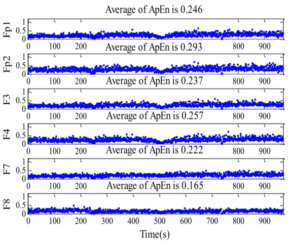
of each channel by ApEn measure(r=0.25) from 0 second to
1030 second. It can be seen from the Fig. 4, comparing with
the first patient, ApEn measure distribution of each channel
is mostly over 0.9, and the average results of each channel
are from 0.972 to 1.22, and gives us a much higher ApEn
value of approximate to 1. According to the definition of
the ApEn, random sequence produces a higher ApEn value
of approximate to 1, we consider this patient’s EEG data is
without spontaneous brain activity. From this result above, we
suspect the patient was in the quasi-brain-death state. Then we
use the MEMD to analysis the patient’s EEG. As showed in
Fig. 5, with the same analysis of the first patient, contrary
to the first patient power spectrum, the value is in a low
range. The average energy of each channel is 0.229×10
4. The
analysis result indicate that this patient physiological brain
activity is extremely low and we suspect the patient was in
the quasi-brain- death state. Later, the clinical doctor confirm
this result is correct.
0 100 200 300 400 500 600 700 800 900 1000 0 0.5 1 1.5 Average of ApEn is 1.17 Fp1 0 100 200 300 400 500 600 700 800 900 1000 0 0.5 1 1.5 Average of ApEn is 0.984 Fp2 0 100 200 300 400 500 600 700 800 900 1000 0 0.5 1 1.5 Average of ApEn is 1.22 F3 0 100 200 300 400 500 600 700 800 900 1000 0 0.5 1 1.5 Average of ApEn is 0.972 F4 0 100 200 300 400 500 600 700 800 900 1000 0 0.5 1 1.5 Average of ApEn is 1.2 C3 0 100 200 300 400 500 600 700 800 900 1000 0 0.5 1 1.5 Average of ApEn is 1.05 Time(s) C4
Fig. 4. Approximate Entropy measure’s distribution and average value of the second Patient. 0 0.5 1 −20 0 20 0 0.5 1 −20 0 20 0 0.5 1 −10 0 10 0 0.5 1 −20 0 20 0 0.5 1 −10 0 10 0 0.5 1 −20 0 20 0 10 20 0 5000 0 10 20 0 5000 0 10 20 0 5000 0 10 20 0 5000 0 10 20 0 5000 0 10 20 0 5000 0 0.5 1 0 20 40 X1 0 0.5 1 −500 50 X2 0 0.5 1 −200 20 X3 0 0.5 1 −200 20 X4 0 0.5 1 −200 20 X5 0 0.5 1 −500 50 X6 0 0.5 1 −50 5 C 1 0 0.5 1 −50 5 0 0.5 1 −50 5 0 0.5 1 −50 5 0 0.5 1 −50 5 0 0.5 1 −50 5 0 0.5 1 −50 5 C 2 0 0.5 1 −50 5 0 0.5 1 −50 5 0 0.5 1 −50 5 0 0.5 1 −50 5 0 0.5 1 −50 5 0 0.5 1 −20 2 C 3 0 0.5 1 −20 2 0 0.5 1 −20 2 0 0.5 1 −50 5 0 0.5 1 −20 2 0 0.5 1 −50 5 0 0.5 1 −50 5 C 4 0 0.5 1 −50 5 0 0.5 1 −50 5 0 0.5 1 −50 5 0 0.5 1 −50 5 0 0.5 1 −50 5 0 0.5 1 −50 5 C 5 0 0.5 1 −50 5 0 0.5 1 −50 5 0 0.5 1 −50 5 0 0.5 1 −50 5 0 0.5 1 −50 5 0 0.5 1 −50 5 C 6 0 0.5 1 −50 5 0 0.5 1 −50 5 0 0.5 1 −50 5 0 0.5 1 −20 2 0 0.5 1 −50 5 0 0.5 1 −50 5 C 7 0 0.5 1 −50 5 0 0.5 1 −50 5 0 0.5 1 −50 5 0 0.5 1 −20 2 0 0.5 1 −50 5 0 0.5 1 −10 1 C 8 0 0.5 1 −10 1 0 0.5 1 −0.50 0.5 0 0.5 1 −20 2 0 0.5 1 −10 1 0 0.5 1 −10 1 0 0.5 1 −0.50 0.5 C 9 0 0.5 1 −10 1 0 0.5 1 −10 1 0 0.5 1 −20 2 0 0.5 1 −0.50 0.5 0 0.5 1 −10 1 0 0.5 1 −20 2 C 1 0 0 0.5 1 −10 1 0 0.5 1 −10 1 0 0.5 1 −20 2 0 0.5 1 −10 1 0 0.5 1 −20 2 0 0.5 1 6 8 10 r 0 0.5 1 4 6 8 0 0.5 1 −20 2 0 0.5 1 0 5 10 0 0.5 1 6 8 10 0 0.5 1 6 7 8
Fig. 5. The second Patient for quasi-brain-death state used MEMD.
D. The EEG Energy of all patients
EEG energy analysis is supplied to evaluate the brain
activity. EEG energy of healthy human is higher than comatose
patient and brain death. However, Fig. 6 show the EEG energy
of all patients. In Fig. 6, healthy human’s maximum EEG
energy of each channel is 7.42×10
4, and the minimum is
0.806×10
4. Contrary to this, brain deaths reflected no EEG
energy over 0.48×10
4. However, comatose patients’ EEG
energy of each channel is between 8.00×10
4and 0.8×10
4.
Fig.3-6 MEMD result of brain death patient 3.1.3 Analysis result based on Dynamic-MEMD method
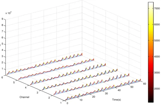
Furthermore, let us show dynamic EEG energy of healthy subject, comatose patient and brain death by using Dynamic-MEMD. By applying the Dynamic-MEMD method, with the change of time, the number of IMF components will change in theory. In our experiments, 5 lower frequency IMF components are combined to form the denoised EEG signal. Therefore, the number of IMF components change will not affect the result of experiments. The example for healthy subject’s EEG examination was performed in August 2013. The EEG recording last over 500 seconds. By applying Dynamic-MEMD algorithms, we obtain EEG energy variation of healthy subject (Fig.3-7) in 60 seconds. EEG energy of each channel are between 1.43×10⁴ and 8.65×10⁴.
0 0.5 1 −500 50 X1 0 0.5 1 −500 50 X2 0 0.5 1 −500 50 X3 0 0.5 1 −500 50 X4 0 0.5 1 −500 50 X5 0 0.5 1 −500 50 X6 0 0.5 1 −50 5 C 1 0 0.5 1 −50 5 0 0.5 1 −50 5 0 0.5 1 −50 5 0 0.5 1 −50 5 0 0.5 1 −50 5 0 0.5 1 −100 10 C 2 0 0.5 1 −50 5 0 0.5 1 −50 5 0 0.5 1 −100 10 0 0.5 1 −50 5 0 0.5 1 −50 5 0 0.5 1 −100 10 C 3 0 0.5 1 −100 10 0 0.5 1 −50 5 0 0.5 1 −100 10 0 0.5 1 −100 10 0 0.5 1 −50 5 0 0.5 1 −50 5 C 4 0 0.5 1 −50 5 0 0.5 1 −50 5 0 0.5 1 −50 5 0 0.5 1 −50 5 0 0.5 1 −50 5 0 0.5 1 −20 2 C 5 0 0.5 1 −50 5 0 0.5 1 −50 5 0 0.5 1 −50 5 0 0.5 1 −50 5 0 0.5 1 −100 10 0 0.5 1 −50 5 C 6 0 0.5 1 −100 10 0 0.5 1 −50 5 0 0.5 1 −50 5 0 0.5 1 −50 5 0 0.5 1 −50 5 0 0.5 1 −200 20 C 7 0 0.5 1 −200 20 0 0.5 1 −50 5 0 0.5 1 −200 20 0 0.5 1 −100 10 0 0.5 1 −100 10 0 0.5 1 −100 10 C 8 0 0.5 1 −100 10 0 0.5 1 −100 10 0 0.5 1 −200 20 0 0.5 1 −50 5 0 0.5 1 −100 10 0 0.5 1 −100 10 C 9 0 0.5 1 −100 10 0 0.5 1 −100 10 0 0.5 1 −100 10 0 0.5 1 −100 10 0 0.5 1 −200 20 0 0.5 1 −100 10 r 0 0.5 1 −100 10 0 0.5 1 −100 10 0 0.5 1 −200 20 0 0.5 1 0 10 20 0 0.5 1 −200 20 0 0.5 1 −20 0 20 0 0.5 1 −50 0 50 0 0.5 1 −20 0 20 0 0.5 1 −50 0 50 0 0.5 1 −20 0 20 0 0.5 1 −50 0 50 0 10 20 0 5000 0 10 20 0 5000 0 10 20 0 5000 0 10 20 0 5000 0 10 20 0 5000 0 10 20 0 5000
Fig. 3. The first Patient for comatose patient used MEMD.
find the value of power spectra at 2-10 Hz is very high. The
average energy of each channel is 2.14×10
4. The analysis
result indicated the patient still had strong physiological brain
activity, and in fact, the patient was in a comatose state.
Furthermore, clinical diagnosis from the doctor confirm the
patient is in a coma state at recorded time.
C. A Patient in the Quasi-Brain-Death State
The second patient’s EEG examination was carried out one
day in June 2010, and was lasted 1030 seconds. Being similar
analysis to the previous, we calculate every 1 second data
of each channel by ApEn measure(r=0.25) from 0 second to
1030 second. It can be seen from the Fig. 4, comparing with
the first patient, ApEn measure distribution of each channel
is mostly over 0.9, and the average results of each channel
are from 0.972 to 1.22, and gives us a much higher ApEn
value of approximate to 1. According to the definition of
the ApEn, random sequence produces a higher ApEn value
of approximate to 1, we consider this patient’s EEG data is
without spontaneous brain activity. From this result above, we
suspect the patient was in the quasi-brain-death state. Then we
use the MEMD to analysis the patient’s EEG. As showed in
Fig. 5, with the same analysis of the first patient, contrary
to the first patient power spectrum, the value is in a low
range. The average energy of each channel is 0.229×10
4. The
analysis result indicate that this patient physiological brain
activity is extremely low and we suspect the patient was in
the quasi-brain- death state. Later, the clinical doctor confirm
this result is correct.
0 100 200 300 400 500 600 700 800 900 1000 0 0.5 1 1.5 Average of ApEn is 1.17 Fp1 0 100 200 300 400 500 600 700 800 900 1000 0 0.5 1 1.5 Average of ApEn is 0.984 Fp2 0 100 200 300 400 500 600 700 800 900 1000 0 0.5 1 1.5 Average of ApEn is 1.22 F3 0 100 200 300 400 500 600 700 800 900 1000 0 0.5 1 1.5 Average of ApEn is 0.972 F4 0 100 200 300 400 500 600 700 800 900 1000 0 0.5 1 1.5 Average of ApEn is 1.2 C3 0 100 200 300 400 500 600 700 800 900 1000 0 0.5 1 1.5 Average of ApEn is 1.05 Time(s) C4
Fig. 4. Approximate Entropy measure’s distribution and average value of the second Patient. 0 0.5 1 −20 0 20 0 0.5 1 −20 0 20 0 0.5 1 −10 0 10 0 0.5 1 −20 0 20 0 0.5 1 −10 0 10 0 0.5 1 −20 0 20 0 10 20 0 5000 0 10 20 0 5000 0 10 20 0 5000 0 10 20 0 5000 0 10 20 0 5000 0 10 20 0 5000 0 0.5 1 0 20 40 X 1 0 0.5 1 −500 50 X 2 0 0.5 1 −200 20 X 3 0 0.5 1 −200 20 X 4 0 0.5 1 −200 20 X 5 0 0.5 1 −500 50 X 6 0 0.5 1 −50 5 C 1 0 0.5 1 −50 5 0 0.5 1 −50 5 0 0.5 1 −50 5 0 0.5 1 −50 5 0 0.5 1 −50 5 0 0.5 1 −50 5 C 2 0 0.5 1 −50 5 0 0.5 1 −50 5 0 0.5 1 −50 5 0 0.5 1 −50 5 0 0.5 1 −50 5 0 0.5 1 −20 2 C 3 0 0.5 1 −20 2 0 0.5 1 −20 2 0 0.5 1 −50 5 0 0.5 1 −20 2 0 0.5 1 −50 5 0 0.5 1 −50 5 C 4 0 0.5 1 −50 5 0 0.5 1 −50 5 0 0.5 1 −50 5 0 0.5 1 −50 5 0 0.5 1 −50 5 0 0.5 1 −50 5 C 5 0 0.5 1 −50 5 0 0.5 1 −50 5 0 0.5 1 −50 5 0 0.5 1 −50 5 0 0.5 1 −50 5 0 0.5 1 −50 5 C 6 0 0.5 1 −50 5 0 0.5 1 −50 5 0 0.5 1 −50 5 0 0.5 1 −20 2 0 0.5 1 −50 5 0 0.5 1 −50 5 C 7 0 0.5 1 −50 5 0 0.5 1 −50 5 0 0.5 1 −50 5 0 0.5 1 −20 2 0 0.5 1 −50 5 0 0.5 1 −10 1 C 8 0 0.5 1 −10 1 0 0.5 1 −0.50 0.5 0 0.5 1 −20 2 0 0.5 1 −10 1 0 0.5 1 −10 1 0 0.5 1 −0.50 0.5 C 9 0 0.5 1 −10 1 0 0.5 1 −10 1 0 0.5 1 −20 2 0 0.5 1 −0.50 0.5 0 0.5 1 −10 1 0 0.5 1 −20 2 C 1 0 0 0.5 1 −10 1 0 0.5 1 −10 1 0 0.5 1 −20 2 0 0.5 1 −10 1 0 0.5 1 −20 2 0 0.5 1 6 8 10 r 0 0.5 1 4 6 8 0 0.5 1 −20 2 0 0.5 1 0 5 10 0 0.5 1 6 8 10 0 0.5 1 6 7 8
Fig. 5. The second Patient for quasi-brain-death state used MEMD.
D. The EEG Energy of all patients
EEG energy analysis is supplied to evaluate the brain
activity. EEG energy of healthy human is higher than comatose
patient and brain death. However, Fig. 6 show the EEG energy
of all patients. In Fig. 6, healthy human’s maximum EEG
energy of each channel is 7.42×10
4, and the minimum is
0.806×10
4. Contrary to this, brain deaths reflected no EEG
energy over 0.48×10
4. However, comatose patients’ EEG
energy of each channel is between 8.00×10
4and 0.8×10
4.
Fig.3-7 EEG energy variation of healthy subject
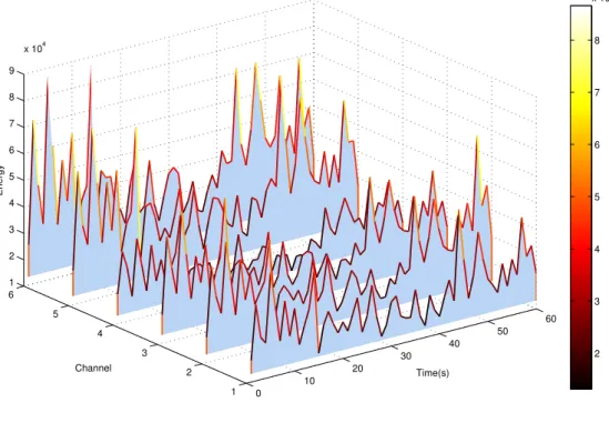
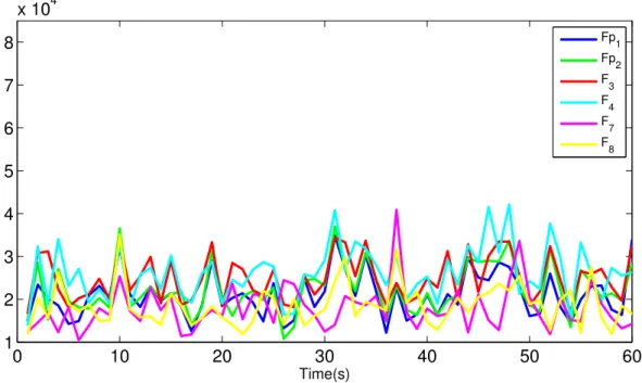
Fig.3-8 EEG energy variation of healthy subject in three-dimensional display The comatose case is concerned with a male patient. The EEG recording lasted 380 seconds. By the same way of healthy subject to analysis the EEG data of this patient by Dynamic-MEMD, we obtain the EEG energy variation of comatose patient in 60 seconds (Fig.3-9). This patient’s EEG energy of each channel is between 1.05×10⁴ to
4.2×10⁴ that reflects a high intensity of brain activity.
0 10 20 30 40 50 60 1 2 3 4 5 6 7 8 9x 10 4 Time(s) Fp 1 Fp2 F3 F 4 F 7 F 8
(a) EEG energy variation of a healthy subject.
0 10 20 30 40 50 60 1 2 3 4 5 6 7 8 x 10⁴ Time(s) Fp 1 Fp 2 F 3 F4 F 7 F 8
(b) EEG energy variation of a comatose patient.
0 10 20 30 40 50 60 0 1 2 3 4 5 6 7 8 x 10⁴ Time(s) Fp 1 Fp2 F 3 F 4 F7 F 8
(c) EEG energy variation of a brain death.
Fig. 2. Results for a dynamic EEG energy analysis using D-MEMD.
subject using MEMD to calculate a static EEG energy. This
subject’s EEG recording last over 500 seconds.
As shown in Fig. 1, the decomposing condition of channel
Fp1, Fp2, F3, F4, F7 and F8 expressed as X
1, X
2, X
3,
X
4, X
5and X
6in the time range one second is selected
randomly. By applying the MEMD method described in
Section II-A, we obtain 7 IMF components (C
1to C
7)
within different frequency from high to low. Since the IMF
components C
1to C
2that with high frequency scales refer
to electrical interference or other noise from environment
that contains in the recorded EEG. The residual component
r
is not the typical useful components considered, either.
The desired components from C
3to C
7are combined to
form the denoised EEG signal, and changed into frequency
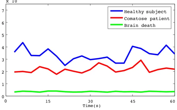
0 5 10 15 20 0 1 2 3 4 5 6 7 x 10⁴ Healthy human Comatose patient Brain death 15 30 45 60 TimesTime(s) subject
Fig. 3. Comparison of dynamic EEG energy for a healthy subject, comatose patient and brain death.
domain by fast Fourier transform (FFT) (Fig. 1). And then
we integrate the denoised signal and calculate the energy
of EEG data. The average energy of every channels of this
second is 6.05⇥10
4.
C. Result for Healthy Subject, Comatose Patient and Brain
Death Using D-MEMD
Furthermore, let us show dynamic EEG energy of healthy
subject, comatose patient and brain death by using
D-MEMD. By applying the D-MEMD method described in
the Section II-B, with the change of time, the number of
IMF components will change in theory. In our experiments,
5 lower frequency IMF components are combined to form
the denoised EEG signal. Therefore, the number of IMF
components change will not affect the result of experiments.
The example for healthy subject’s EEG examination was
performed in August 2013. The EEG recording last over
500 seconds. By applying D-MEMD algorithms described
in Section II-B, we obtain EEG energy variation of healthy
subject (Fig. 2-a) in 60 seconds. EEG energy of each channel
are between 1.43⇥10
4and 8.65⇥10
4.
The comatose case is concerned with a male patient. The
EEG recording lasted 380 seconds. By the same way of
healthy subject to analysis the EEG data of this patient by
D-MEMD, we obtain the EEG energy variation of comatose
patient in 60 seconds (Fig. 2-b). This patient’s EEG energy
of each channel is between 1.05⇥10
4to 4.2⇥10
4(Fig. 2-b)
that reflects a high intensity of brain activity.
With the same analysis for brain death, we still analyzed
60 seconds EEG data by using D-MEMD as an example. Fig.
2-c shows each channel’s EEG energy. This patient’s
max-imum value of 6 channels’ EEG energy is only 7.03⇥10
3,
the value is extremely low. The analysis result indicate that
this patient’ physiological brain activity is extremely low.
D. Comparison of EEG Energy for Healthy Subject,
Co-matose Patient and Brain death
Fig. 5 shows the Comparison of total EEG energy for
healthy subject, comatose and brain death by simple moving
average for 3 seconds. First, we averaged each channel’s
EEG energy of these 3 subjects. Moreover, by using simple
moving average, we averaged 3 seconds’ EEG energy of each
Fig.3-9 EEG energy variation of coma subject
Fig.3-10 EEG energy variation of coma subject in three-dimensional display With the same analysis for brain death, we still analyzed 60 seconds EEG data by using Dynamic-MEMD as an example. Fig.3-11 shows each channel’s EEG energy. This patient’s maximum value of 6 channels’ EEG energy is only 7.03×10³, the value
is extremely low. The analysis result indicates that this patient’ physiological brain
0 10 20 30 40 50 60 1 2 3 4 5 6 7 8 9x 10 4 Time(s) Fp1 Fp2 F3 F4 F7 F8
(a) EEG energy variation of a healthy subject.
0 10 20 30 40 50 60 1 2 3 4 5 6 7 8 x 10⁴ Time(s) Fp 1 Fp2 F3 F 4 F7 F 8
(b) EEG energy variation of a comatose patient.
0 10 20 30 40 50 60 0 1 2 3 4 5 6 7 8 x 10⁴ Time(s) Fp 1 Fp 2 F 3 F 4 F 7 F 8
(c) EEG energy variation of a brain death.
Fig. 2. Results for a dynamic EEG energy analysis using D-MEMD.
subject using MEMD to calculate a static EEG energy. This
subject’s EEG recording last over 500 seconds.
As shown in Fig. 1, the decomposing condition of channel
Fp1, Fp2, F3, F4, F7 and F8 expressed as X
1, X
2, X
3,
X
4, X
5and X
6in the time range one second is selected
randomly. By applying the MEMD method described in
Section II-A, we obtain 7 IMF components (C
1to C
7)
within different frequency from high to low. Since the IMF
components C
1to C
2that with high frequency scales refer
to electrical interference or other noise from environment
that contains in the recorded EEG. The residual component
r
is not the typical useful components considered, either.
The desired components from C
3to C
7are combined to
form the denoised EEG signal, and changed into frequency
0 5 10 15 20 0 1 2 3 4 5 6 7 x 10⁴ Healthy human Comatose patient Brain death 15 30 45 60 TimesTime(s) subject
Fig. 3. Comparison of dynamic EEG energy for a healthy subject, comatose patient and brain death.
domain by fast Fourier transform (FFT) (Fig. 1). And then
we integrate the denoised signal and calculate the energy
of EEG data. The average energy of every channels of this
second is 6.05⇥10
4.
C. Result for Healthy Subject, Comatose Patient and Brain
Death Using D-MEMD
Furthermore, let us show dynamic EEG energy of healthy
subject, comatose patient and brain death by using
D-MEMD. By applying the D-MEMD method described in
the Section II-B, with the change of time, the number of
IMF components will change in theory. In our experiments,
5 lower frequency IMF components are combined to form
the denoised EEG signal. Therefore, the number of IMF
components change will not affect the result of experiments.
The example for healthy subject’s EEG examination was
performed in August 2013. The EEG recording last over
500 seconds. By applying D-MEMD algorithms described
in Section II-B, we obtain EEG energy variation of healthy
subject (Fig. 2-a) in 60 seconds. EEG energy of each channel
are between 1.43⇥10
4and 8.65⇥10
4.
The comatose case is concerned with a male patient. The
EEG recording lasted 380 seconds. By the same way of
healthy subject to analysis the EEG data of this patient by
D-MEMD, we obtain the EEG energy variation of comatose
patient in 60 seconds (Fig. 2-b). This patient’s EEG energy
of each channel is between 1.05⇥10
4to 4.2⇥10
4(Fig. 2-b)
that reflects a high intensity of brain activity.
With the same analysis for brain death, we still analyzed
60 seconds EEG data by using D-MEMD as an example. Fig.
2-c shows each channel’s EEG energy. This patient’s
max-imum value of 6 channels’ EEG energy is only 7.03⇥10
3,
the value is extremely low. The analysis result indicate that
this patient’ physiological brain activity is extremely low.
D. Comparison of EEG Energy for Healthy Subject,
Co-matose Patient and Brain death
Fig. 5 shows the Comparison of total EEG energy for
healthy subject, comatose and brain death by simple moving
average for 3 seconds. First, we averaged each channel’s
EEG energy of these 3 subjects. Moreover, by using simple
moving average, we averaged 3 seconds’ EEG energy of each
activity is extremely low.
Fig.3-11 EEG energy variation of brain death subject
Fig.3-12 EEG energy variation of brain death subject in three-dimensional display
Fig. 3-13 shows the Comparison of total EEG energy for healthy subject, comatose and brain death by simple moving average for 3 seconds. First, we averaged each channel’s EEG energy of these 3 subjects. Moreover, by using simple moving average,
0 10 20 30 40 50 60 1 2 3 4 5 6 7 8 9x 10 4 Time(s) Fp 1 Fp 2 F 3 F 4 F 7 F8
(a) EEG energy variation of a healthy subject.
0 10 20 30 40 50 60 1 2 3 4 5 6 7 8 x 10⁴ Time(s) Fp 1 Fp 2 F 3 F 4 F7 F 8
(b) EEG energy variation of a comatose patient.
0 10 20 30 40 50 60 0 1 2 3 4 5 6 7 8 x 10⁴ Time(s) Fp1 Fp 2 F3 F 4 F7 F 8
(c) EEG energy variation of a brain death.
Fig. 2. Results for a dynamic EEG energy analysis using D-MEMD.
subject using MEMD to calculate a static EEG energy. This
subject’s EEG recording last over 500 seconds.
As shown in Fig. 1, the decomposing condition of channel
Fp1, Fp2, F3, F4, F7 and F8 expressed as X
1, X
2, X
3,
X
4, X
5and X
6in the time range one second is selected
randomly. By applying the MEMD method described in
Section II-A, we obtain 7 IMF components (C
1to C
7)
within different frequency from high to low. Since the IMF
components C
1to C
2that with high frequency scales refer
to electrical interference or other noise from environment
that contains in the recorded EEG. The residual component
r
is not the typical useful components considered, either.
The desired components from C
3to C
7are combined to
form the denoised EEG signal, and changed into frequency
0 5 10 15 20 0 1 2 3 4 5 6 7 x 10⁴ Healthy human Comatose patient Brain death 15 30 45 60 TimesTime(s) subject
Fig. 3. Comparison of dynamic EEG energy for a healthy subject, comatose patient and brain death.