EVALUATION OF JOINING STRENGTH OF SILICON-RESIN INTERFACE AT A VERTEX IN 3D JOINT STRUCTURE

EVALUATION OF JOINING STRENGTH OF SILICON-RESIN INTERFACE AT A VERTEX IN 3D JOINT STRUCTURE

Hideo KOGUCHI

Department of Mechanical Engineering Nagaoka University of Technology Nagaoka, Niigata 940-2188, Japan E-mail: [email protected]

Kazuhisa HOSHI

Department of Mechanical Engineering

Graduate School of Nagaoka University of Technology Nagaoka, Niigata 940-2188, Japan

E-mail: [email protected]

ABSTRACT

Portable electric devices such as mobile phone and portable music player become compact and improve their performance. High-density packaging technology such as CSP (Chip Size Package) and Stacked-CSP is used for improving the performance of devices. CSP has a bonded structure composed of materials with different properties.

A mismatch of material properties may cause stress sin- gularity, which lead to the failure of bonding part in structures.

In the present paper, stress analysis using boundary element method and an eigenvalue analysis using finite element method are used for evaluating the intensity of singularity at a vertex in three-dimensional joints.

Three-dimensional boundary element program based on the fundamental solution for two-phase isotropic materi- als is used for calculating the stress distribution in a three-dimensional joint. Angular function in the singular stress field at the vertex in the three-dimensional joint is calculated using eigen vector determined from the eigen- value analysis.

The joining strength of interface in several kinds of sillicon-resin specimen with different triangular bonding areas is investigated analytically and experimentally. Ex- periment for debonding the interface in the joints is firstly

carried out. Stress singularity analysis for the three-dimensional joints subjected to an external force for debonding the joints is secondly conducted. Combining results of the experiment and the analysis yields a final stress distribution for evaluating the strength of interface.

Finally, a relationship of force for delamination in joints with different bonding areas is derived, and a critical val- ue of the 3D intensity of singularity is determined.

INTRODUCTION

CSP is used in recent electronic devices for improving their functionality and performance. CSP is consisted of IC chip, resin and metals, and delamination occurs fre- quently at a vertex of interface between IC and resin. A lot of studies on the joints have been carried out theoreti- cally and experimentally[1]-[3]. In the previous study, two-dimensional joints are extensively investigated, however, few studies on three-dimensional joint struc- tures have been carried out until now[4]. Real CSP has a three-dimensional shape and an interface. Therefore, it is necessary to evaluate strength of interface at the vertex in three-dimensional joints.

Generally, singular stress fields at the edge of inter- face in joints can be described as σij=ΣmK_ij^m f_ij^m(θ,φ)r^-λm, Proceedings of the ASME 2011 Pacific Rim Technical Conference & Exposition on

Packaging and Integration of Electronic and Photonic Systems InterPACK2011 July 6-8, 2011, Portland, Oregon, USA

InterPACK2011-52065 IPACK2011-

where r represents the distance from the origin of singular stress field, λm the order of stress singularity, !_!"^! the intensity of singularity for stresses !_!", !_!"^! !,! angu- lar functions. In the case of 0<λm<1, it can be said that the stress field has a stress singularity [5]-[9].

In the present paper, a simple specimen is used for investigating the strength of interface at the vertex in a Si-resin joint constituting CSP. Firstly, the order of stress singularity is derived from eigenvalue analysis based on FEM, and an angular function for the singular stress field at the vertex in three-dimensional joints is calculated us- ing eigen vector determined from the eigen analysis.

Secondly, a stress analysis is performed using BEM under mechanical and thermal loadings. It will be shown that residual thermal stress in the specimen is very small. Fi- nally, the bonding strength of the interface is estimated experimentally and theoretically. A relationship between the bonding strength in joints and the bondibg areas is derived. The critical intensity of stress singularity on the interface in three-dimensional joints is determined to es- timate the strength of interface.

ANALYSIS METHODS FOR SINGULAR STRESS FIELD

Three-dimensional boundary element method The boundary integral equation can be expressed as follows.

!_!" ! !_! ! = !_!" !,! !_! !

!

−!_!" !,! !_! ! !" !      (1)

where c_ij(P) represents a constant depending on the shape of boundary, P and Q are an observation point and a source point locating on the boundary Γ , and U_ij and T_ij represent the fundamental solutions for displacement and traction. Here, Rongved's solution which is the Green function for two-phase isotropic materials is used as the fundamental solution for calculating the stress fields at the vertex in three-dimensional joints. Stress distribution in the domain for analysis is evaluated using Hooke's law and the following equation.

!_!,! ! = !_!",! !,! !_! !

! −!_!!,! !,! !_! ! !" !      (2)

where U_ij,k and T_ij,k are the derivatives of fundamental solutions of displacement and traction with respect to P.

Boundary element method does not require so many data as finite element method does. Using the fundamen- tal solutions for two-phase materials, mesh division on the interface is not therefore needed. Hence, stress distribu- tion on the interface near the vertex can be calculated precisely.

Eigen analysis

The order of stress singularity, λ, which characterizes stress field is determined using an eigen equation which is formulated on the basis of finite element method as fol- lows (see Pageau & Biggers [10]).

(p²[A]+ p[B]+[C]){u}= 0 (3) where λ=1-Re(p), p is a root of Eq.(3), [A], [B] and [C]

are matrices consisted of elastic moduli and the geometry of joints, {u} represents a nodal displacement vector.

When 0<λ<1, the stress field has a stress singularity, and when l >0, the stress singularity disappears.

DELAMINATION EXPERIMENTS Material and method

In the present study, specimens which two IC (silicon) square plates are bonded using an underfill resin are pre- pared as shown in Fig.1. This type of specimen was de- veloped for investigating the strength of interface at the 3D vertex in multi-layered thin films by Shibutani[11].

The silicon plate is a square of 6mm×6mm and 0.63mm in thickness. The resin is a square of 3mm×6mm and 0.05mm in thickness. The specimens have triangular bonding area. Experiment for delamination is carried out under conditions that the bonding area A varied about from 0.50mm² to 2.0mm². In a bonding process, the specimen is heated up 453K and two silicon plates are bonded to each other with resin. After that, it is naturally cooled to room temperature. The specimen is kept in a desiccator until delamination test.

A schematic view of experimental apparatus is shown in Fig.2(A) and a portion encircled in this figure is en- larged and shown in Fig.2(B). A tensile load testing ma- chine is used for delamination test. A load cell is attached at one end of the machine for measuring the force of de- lamination in specimens, which are glued at Jig2 as shown in Fig.2(B). Delamination test is carried out in the way that a specimen is pushed with a small steel ball of 2mm in diameter glued to Jig1 attached to a rod of the load cell in the arrow direction.

Fig.1 Shape of specimen 5.0

3.0 6.0

6.0

0.63 0.63 Interface

Silicon Resin Silicon

point Load r

φ

unit : mm

O

A=0.49, 1.0, 1.9881, 2.9929mm² D=0.7, 1.0,

1.41, 1.73

t=0.05 A=0.49, 1.0, 1.99 mm²

D =

0.7, 1.0, 1.41 mm

Results

A crack ran brittlely along an interface from the three- dimensional corner. Delamination surface was the inter- face between silicon and resin. The delamination occurred at the interface between the upper silicon and the resin.

Through the precise observation of the fracture surface, it was found that the delamination initiated at the vertex of the joint. Hence, we perform stress analyses at the vertex of upper interface bonding silicon and resin.

The results of the delamination test for each condition are shown in Fig.3. Delamination forces are shown in Fig.3(A), and delamination stresses which are divided each load by each bonding area are shown in Fig.3(B).

Average forces for the bonding area of 0.5mm², 1.0mm² and 2.0mm² are 0.59N, 1.27N and 3.34N, respectively.

Average of delamination stress is 1.20MPa, 1.27MPa and 1.68MPa, respectively. Hence, it is found that delamina- tion force decreased with decreasing the bonding area.

These experimental results are shown in Table 1.

Table.1 Experimental results

Bonding area, mm²

Delamination force F, N

Delamination stress, MPa Lower Average Upper Lower Average Upper 0.49 0.42 0.59 0.74 0.85 1.20 1.51

1.0 1.10 1.27 1.55 1.10 1.27 1.55 1.99 2.66 3.34 4.38 1.33 1.68 2.20

THERMAL DEFORMATION EXPERIMENTS In bonding process of two silicon specimens by resin, the specimens are heated up to 435K and naturally cooled down to room temperature. Hence, residual thermal stress maybe occur in the specimen. Here, warpage in the specimen before and after bonding is measured using a laser measurement system whether residual thermal stress exists or not. Schematic view of the laser measurement

Test part load cell

Specimen Steel ball Jig 1

Jig2

(A) Testing apparatus (B) Enlargement of test part Fig.2 Schematic view of delamination test

(A) Delamination forces (B) Delamination stresses Fig.3 The comparison of experimental results

5.0 4.0 3.0 2.0 1.0 0.0

Delamination force F, N

2.0 1.5

1.0 0.5

Bonding area A, mm²

Delamination force Average

2.5 2.0 1.5 1.0 0.5 0.0

Delamination stress, MPa

2.0 1.5

1.0 0.5

Bonding area A, mm²

Delamination stress Average

system is shown in Fig.4. The specimen put on XY-Stage moves under the laser measurement system, and the warpage of specimens is measured. The specimen with bonding area of A=1.0mm² was measured. The warpage along Line ST passing through the vertex of upper silicon shown in Fig.5 was measured.

Figure 6 represents the result of the measurement and the warpage along Line S calculated from thermal residu- al stress analysis using boundary element method. It is found that the specimen did not deform before and after heating. We suppose that residual thermal stress released after bonding. Hence, thermal residual stress little influ- ences on the delamination force.

Fig.4 Schematic view of a measurement

Fig.5 Scan line for a measurement

ANALYSIS OF STRESS SINGULARITY Eigen analysis

In the experiment, delamination occurs at the vertex of the upper interface between silicon and resin, so eigen analysis at the vertex is performed. A model for eigen analysis is shown in Fig.7, where angles around the stress singularity point O are φ1=90º, φ2=360º, and angles around the stress singularity line are φ1=180º, φ2=360º.

Firstly, the order of stress singularity is determined using Eq.(3). The mesh division for eigen analysis is shown in Fig.8. This figure represents a developed mesh on the θ-φ plane of the sphere surface shown in Fig.5. In this analysis, mesh size of θ and φ coordinates is θ×φ=15^o×15^o and a mesh involving an interface and stress singularity lines is equally divided by five θ×φ=3^o×3^o. Material properties used in the analysis are shown in Ta- ble 2.

Fig.6 Measurements and analysis results for the thermal deformation Resin

upper surface

of resin e r

q

Silicon

O q₁ q₂

Stress singularity line

Stress singularity point

Fig.7 Spherical coordinate system with an origin at a vertex

60 40 20 0 -20

Wargape,µm

6000 5000

4000 3000

2000 1000

0 DistancefromedgeS,µm

Beforeheating(BEM) AfterHeating(BEM)

Beforeheating(measurements) Afterheating(measurements)

Fig.8 A mesh of the developed θ ×φ plane (φ1=180^o and φ2=360^o model)

Results of eigen analysis are shown in Table 3. It is found that several eigen values yielding stress singularity exist for each pair of the angles, φ1 and φ2, of vertex. In the previous study on the three-dimensional stress singu- larity[12], when a triple root of p=1 exists, logarithmic singularity occurs at the stress field. Then, the stress field at the vertex in three-dimensional joints can be expressed as follows.

!_!" !,!,! =!_!!"!_!!" !,! !^!!!"#$"%

+!_!!"!_!!" !,! + !_!"#!_!"# !,!

!

!!!

ln! ^!!!      (4)

where M=4 (with a triple root of p=1), 5 (with a qu adruple root of p=1.0). λvertex represents the order of stress singularity at the vertex. Here, angular function

f_1ij (θ,φ) can be obtained from the eigen vector ({u}

on Eq.(3)) corresponding to eigen value p.

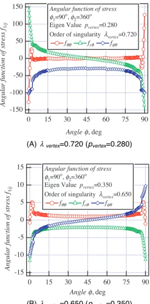
Angular functions at the interface for each eigen value of pvertex=0.280 and 0.350 in the joint angle φ1=90^o, φ2=360^o is shown in Fig.9. In particular, the distribution of f_1θθ(π/2,φ) relating to delamination at the interface is investigated. Here, f_1θθ(π/2,φ) is expressed as f_1θθ^φ(φ).

Table 2 Material properties for analysis

The angular functions are normalized by the value of f_1θθ^φ(φ) at φ=45^o. Here, the value of λvertex for which f1ijφ(φ) is similar to that of σ_ij(r,θ,φ) on the interface against the angle φ obtained by boundary element method is selected.

Then, the order of stress singularity of λ ^vertex=0.65 at the vertex with angles of φ1=90^o, φ2=360^o is selected. The re- sult for boundary element analysis will be shown in the next chapter.

For the order of stress singularity at a point on the singular stress line of φ1=180^o and φ2=360^o, λ ^line=0.49 is selected from a comparison of f_1ij^φ(φ) with σ_ij(r,π/2,φ). Angular function f_1θθ(θ,φ) in the singular stress field can be expressed as follows [13].

!_!!! !

2,! =!_!!!!_!^!!!"#$+!_!!!

+ !!""

!

!!!

ln !_! ^!!!      (5)

where ρΑ is the distances from the singular stress line, and it is expressed as ρ sinφ. Here, ρ is taken to 1.

Singular stress point Singular stress line Joint angle

φ1=90^o, φ2=360^o

Joint angle φ1=180^o, φ2=360^o pvertex

λ ^vertex pline

λ ^line

Real Imaginary Real Imaginary

1 0.280 0.000 0.720 0.514 -0.051 0.486

2 0.350 -0.005 0.650 0.514 0.051 0.486

3 0.350 0.005 0.650 0.507 0.000 0.493

4 1.000 0.000 0.000 1.000 0.000 0.000

5 1.000 0.000 0.000 1.000 0.000 0.000

6 1.000 0.000 0.000 1.000 0.000 0.000

7 - - - 1.000 0.000 0.000

Material Young’s modulus,

GPa Poisson’s ratio

Silicon 169.1 0.26

Resin 2.97 0.38

0 //2

//2

/

/

e

2/ q

Interface

Table 3 List of eigen values and the order of stress singularity for joints

(A) λvertex=0.720 (pvertex=0.280)

(B) λvertex=0.650 (pvertex=0.350)

Fig.9 Angular function of stress f1ijφ(φ) against angle φ (vertex : φ1=90^o and φ2=360^o)

Fig.10 Distributions of stress σθθ, at φ=45 ^o on the interface against r and fitted curve

Table 4 Coefficients in Eq.(6)

Bonding area A, mm² K_1θθ K_2θθ

0.49 13.8 -41.6

1.0 4.82 -21.4

1.99 1.53 -4.67

2.99 0.554 -1.22

Three-dimensional boundary element method Stress analysis using BEM is conducted to determine the intensity of singularity at the vertex in the specimen shown in Fig.1. Domain method is employed in the BEM analysis. Boundary condition is set as the same as delam- ination test, and a unit normal force to the specimen is applied to a point (see Fig.1). Eight nodes quadrilateral serendipity element is used, and the minimum length of side in an element near the vertex is about 10^-6mm. Mate- rial properties used in the analysis are shown in Table 2.

All stress components are transformed from a Carte- sian coordinate system to a spherical coordinate system.

Here, the results of analysis for mechanical loading will be presented for the joints with bonding areas of A=0.49, 1.0, 1.99, 2.99 mm².

Only σθθ of stress components which influence on delamination of the interface will be shown. Distribution of stress, σ_θθ, on the interface against distance from origin r at φ =45^o is shown in Fig.10. It is found that the stress, σ_θθ, decreases with increasing the bonding area. The ex- pression of stress distribution, Eq.(4), can be rewritten as follows.

!_!! !,! 2,!    

=!_!!!!_!!! !

2,! !^!!!"#$"%+!_!!!!_!!! !

2,!        (6)

Here, the logarithmic terms are neglected for simplicity.

Because, it was shown in [14] that the logarithmic terms affect on the stress distribution far from the vertex, and the power law singularity represented by a line in the double logarithmic plot was dominant in this analysis.

The coefficients determined by a least square method us- ing Eq.(6) are shown in Table 4. Where the angular func- tion is normalized to f_1θθ(!/2,φ)=1 at the angle φ =45^o. K_1θθ is the intensity of singularity with respect to the radi- al direction from the vertex. It is found that the value of intensity of singularity K_1θθ decreases with increasing the bonding area.

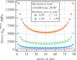
Distribution of stress, σ_θθ, at r=0.0001mm on the in- terface (θ=90^o) against φ is shown in Fig.11. It is found that the stress, σ_θθ, decreases with increasing the bonding area. Figure 12 shows a stress distribution normalized by the value of σ_θθ at the angle φ =45^o. It is found that all dis- tributions are overlapped with each other. Omitting the logarithmic term, the expression of stress distribution can be expressed as follows.

-150 -100 -50 0 50 100 150

Angular function of stress f1ij

90 75 60 45 30 15 0

Angle , deg Angular function of stress

1=90^o, ₂=360^o

Eigen Value p_vertex=0.280 Order of singularity _vertex=0.720

f f_r f

-15 -10 -5 0 5 10 15

Angular function of stress f1ij

90 75 60 45 30 15 0

Angle , deg Angular function of stress

1=90^o, ₂=360^o

Eigen Value p_vertex=0.350 Order of singularity _vertex=0.650

f f_r f

10¹ 10² 10³ 10⁴

Stress Mech , MPa

10^-5 10^-4 10^-3 10^-2 10^-1 Distance from origin r, mm

Mechanical load

=45º, =90º Bonding area A, mm²

0.49 1.0 1.99 2.99 Curve fitting

Fig.11 Distributions of stress σ_θθ, at r =0.0001mm on the interface against φ

Fig.12 Normalized stress

σ

/σ

|

Fig.13 Distributions of critical stress σθθ critical, at φ=45 ^o on the interface against r

Table 5 Coefficients in Eq.(7)

Bonding area A, mm² L_1θθ L_2θθ

0.49 0.535 0.309

1.0 0.532 0.318

1.99 0.511 0.347

2.99 0.503 0.360

!_!!!^! ! =!_!!!!_!^!!!"#$+!_!!!      (7) The coefficients, L_1θθ and L_2θθ, determined by a least square method using Eq.(7) are shown in Table 5. L_1θθ is the intensity of singularity relating to the singular stress line. It is found that L_1θθ a little decreases with increasing the bonding area.

THREE-DIMENSIONAL INTENSITY OF SIINGULARITY

The stress distributions in the singular stress field for a critical status can be expressed by multiplied the stress distributions for a unit load by the delamination force F shown in Table 2. The critical stress, σθθ critical is expressed as follows.

!!!  !"#$#!%&   !,!

2,! =!_!! !,!

2,! !      (8) The stress distribution, σθθ critical, for the critical status is shown in Fig.13. It is found that all plots for different bonding areas are almost overlapped.

Substituting the equation, which f_1θθ in Eq.(6) is re- placed by Eq.(7), into Eq.(8) yields the following equa- tion.

     !!!  !"#$#!%&   !,!

2,!

= !_!!!!_!!!^! ! !^!!!"#$"%+!_!!!!_!!!^! ! !

= !_!!! !_!!!!_!^!!!"#$

+!_!!! !^!!!"#$"%+!_!!!!_!!!^! ! !      (9) Equation (9) is factorized by a coefficient of power law term. Thus,

!!!  !"#$#!%&   !,! 2,!

=!_!!!!_!!!! 1+ !_!!!

!_!!!!_!^!!!"#$

+ !_!!!!_!!!^! !

!_!!!!_!!!!_!^!!!"#$!^!!!"#$"% !_!^!!!"#$!^!!!"#$"%      (10) Here,

!→0°        !ℎ!"         1

!_!^!!!"#$→ !"#$ ^!!"#$ ⟶0

!→0      !ℎ!"        !^!!"#$"%→0 Therefore,

15000 12500 10000 7500 5000 2500 0 Stress Mech , MPa

90 75 60 45 30 15 0

Angle , deg

Mechanical load r=0.0001mm, =90º Bonding area A, mm²

0.49 1.0 1.99 2.99

1

2 3

Normalized stress Mech / Mech |=45º

2 3 4 5 6 7

10 ^{2 3 4 5 6 7}

Angle , deg

Mechanical load r=0.0001mm, =90º Bonding area A, mm²

0.49 1.0 1.99 2.99 Curve fitting

W

W

W W

10¹ 10² 10³ 10⁴

Criticalstress critical,MPa

10^-5 10^-4 10^-3 10^-2 10^-1 Distancefromoriginr,mm

Mechanical load

=45º, =90º Bonding area A, mm² 0.49

1.0 1.99

!!!  !"#$#!%&   !,!

2,!      (11)

=!_!!!!_!!!!!_!^!!!"#$!^!!!"#$"%

Here, ρΑ= sinθ, λ line=0.49 and λ vertex=0.65, therefore,

!!!  !"#$#!%&   !,!

2,!      (12)

=!_!!!!_!!!!sin!^!!.!"!^!!.!"

Coefficients in Eq.(12) is used to evaluate the strength of interface in delamination test. Hence, a critical intensity of singularity is expressed as follows.

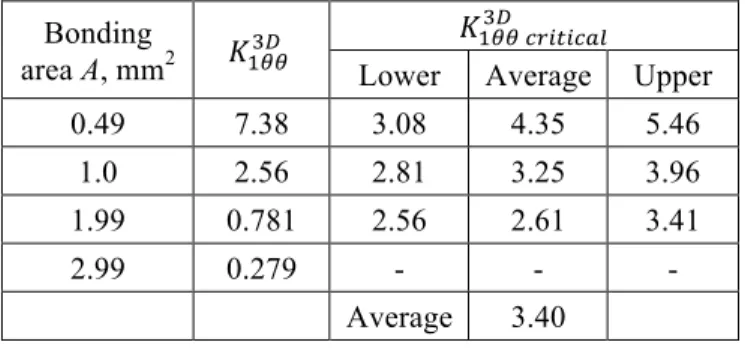
!!!!  !"#$#!%&!! =!_!!!^!!!      (13) Where  !_!!!^!! =!_!!!!_!!! and F is the force for delamina- tion shown in Table 1. !!!!  !"#$#!%&!! is defined as the three-dimensional critical intensity of singularity at the vertex. The values of !_!!!^!!  and !!!!  !"#$#!%&!! are shown in Table 8. It is found that the !!!!  !"#$#!%&!! decreases a little with increasing the bonding area. Considering a var- iation in the result of delamination experiment, a critical value can be determined as the value of !!!!  !"#$#!%&!! . The value of !!!!"#$%$"&'!! for the bonding joints in the present study is between 2.61 and 4.35 MPa•mm^0.65.

CONCLUSION

In the present paper, the strength of interface in three-dimensional joints with several values of the bonding area was evaluated by experiment, BEM and eigen analysis. The critical strength of interface was evaluated from singular stress fields. As a result, the fol- lowing items were obtained.

(1) Warpage of the specimen used in experiment after bonding could be ignored. So, residual thermal stress was not taken into account in evaluating the strength of joint.

(2) Angular functions for several values of the order of stress singularity were derived from eigen analysis, and the expressions for stress distribution were determined comparing the angular functions and the stress distribu- tion obtained by BEM.

(3) An expression for the critical strength of interface was derived for mechanical loading. The critical strength of interface obtained in the present study was about

!!!!  !"#$#!%&!! =2.61~4.35 MPa•mm^0.65.

Table 8 Three-dimensional intensity of singularity Bonding

area A, mm² !_!!!  ^!! !!!!  !"#$#!%&!!

Lower Average Upper

0.49 7.38 3.08 4.35 5.46

1.0 2.56 2.81 3.25 3.96

1.99 0.781 2.56 2.61 3.41

2.99 0.279 - - -

Average 3.40

REFERENCES

[1] Inoue, T. and Koguchi, H. 1996, "Influence of the In- termediate Material on the Order of Stress Singularity in Three-Phase Bonded Structure", Int. J. Solids Structures, Vol.33, pp.399-417.

[2] Qian, Z. Q. and Akisanya, A. R., 1999, "An Investiga- tion of the Stress Singularity near the Free Edge of Scarf Joints", Eur. J. Mech. A/Solids, Vol.18, pp.443-463.

[3] Reedy, JR. and Guess, T. R., 1997, "Interface corner failure analysis of joint strength: Effect of adherend stiff- ness", Int. J. Fracture, Vol.88, pp.305-314.

[4] Koguchi, H. and Muramoto, T., 2000, "The Order of Stress Singularity near the Vertex in Three-Dimensional Joints", Int. J. Solids Structures, Vol.37, pp.4737-4762.

[5] Bogy, D.B., 1970, "On the Problem of Edge-Bonded Elastic Quarter-Planes Loaded at the Boundary", Int. J.

Solids Structures, Vol.6, pp.1287-1313.

[6] Bogy, D.B., 1971, "Two Edge-Bonded Elastic Wedges of Different Materials and Wedge Angles under Surface Tractions", J.Appl. Mech., Vol.38, pp.377-386.

[7] Bogy, D.B., 1971, "On the Plain Elastostatic Problem of a Loaded Crack Terminating at a Material Interface", J.

Appl. Mech. Vol.38, pp.911-918.

[8] Bogy, D.B. and Wang, K.C., 1971, "Stress Singulari- ties at Interface Corners in Bonded Dissimilar Isotropic Elastic Materials", Int. J. Solids Structures, Vol.7, pp.993-1005.

[9] Dempsey, J.P. and Sinclair, G.B., 1979, "On the Stress Singularities in the Plane Elasticity of the Composite Wedge", J. Elasticity, Vol.9, pp.373-391.

[10] Pageau, S. S. and Bigger, Jr S. B., 1995, "Finite El- ement Evaluation of Free-Edge Singular Stress Fields in Anisotropic Materials", Int. J. Numer. Methods Eng, Vol.38, pp.2225-2239.

[11] Shibutani, T., Tsuruga, T., Yu. Q. and Shiratori, M., 2003, “Criteria of Crack Initiation at Edge of Interface between Thin Films in Opening and Sliding Modes for an Advanced LSI”, Trans. Jpn. Soc. Mech. Eng., Vol.69, pp.1368-1373.

[12] Monchai, P., and Koguchi, H., 2007, "Boundary El- ement Analysis of the Stress Field at the Singularity Lines in Three- Dimensional Bonded Joints under Thermal Loading", J. Mechanics of Materials and Structures, Vol.2, No.1, pp.149- 166.

[13] Koguchi, H. and Taniguchi, T., 2008, "Characteris- tics of Stress Singularity Field of Residual Thermal Stresses at vertex in Three-Dimensional Bonded Joints", Trans. the Japan Soc. Mech. Eng., Ser. A, Vol.74, No.724, pp.864-872.

[14] Koguchi, H. and Meo, N., 2006, "An Evaluation of Interface Strength at a Vertex in a Three-Dimensional Joint Considering Residual Thermal Stresses Using Three Dimensional Boundary Element Method", Trans. Jpn. Soc.

Mech. Eng. Vol.72, No.723, pp.1598-1606.