EVALUATION OF THE BONDING STRENGTH AT THE THREE-DIMENSIONAL VERTEX IN SILICON-RESIN JOINTS

EVALUATION OF THE BONDING STRENGTH AT THE THREE-DIMENSIONAL VERTEX IN SILICON-RESIN JOINTS

Hideo KOGUCHI

Department of Mechanical Engineering Nagaoka University of Technology Nagaoka, Niigata 940-2188, Japan E-mail : [email protected]

Masato NAKAJIMA

Department of Mechanical Engineering Graduate School of Nagaoka University of Technology

Nagaoka, Niigata 940-2188, Japan E-mail : [email protected]

IPAC2009-89091

ABSTRACT

Portable electric devices such as mobile phone and portable music player become compact and also their performance improves. High density packaging technology such as CSP (Chip Size Package) and Stacked-CSP is needed to realize advanced functions. CSP is a bonded structure composed of materials with different properties. A mismatch of material properties may cause stress singularity at the edge of interface, which lead to the failure of bonding part in structures.

Singular stress field in residual thermal stresses occurs in a cooling process after bonding the joints at a high temperature.

In the present paper, the strength of interface in CSP consisted of silicon and resin is investigated. Boundary element method and an eigen value analysis based on finite element method are used for evaluating the intensity of singularity of residual thermal stresses at a vertex in a three-dimensional joint. Three-dimensional boundary element program based on the fundamental solution for two-phase isotropic body is used for calculating the stress distribution in the three- dimensional joint. Angular function in the singular stress field at the vertex in the three-dimensional joint is calculated using eigen vector determined from eigen analysis. The strength of bonding at the interface in several silicon-resin specimens with different thickness of resin is investigated analytically and experimentally. Stress singular analysis applying an external force for the joints is firstly carried out. After that,

singular stress field for the residual thermal stresses varying material property of resin with temperature is calculated.

Combining singular stress fields for the external force and the residual thermal stress yields a final stress distribution for evaluating the strength of interface. A relationship between the external force for delamination in joints and the thickness of resin is derived. Finally, a critical intensity of singularity for delamination between silicon and resin is determined.

INTRODUCTION

CSP is used in recent electronic devices for improving its functionality and performance. CSP is consisted of IC chip, resin and metals, and delamination occurs frequently at an interface between IC and resin. A lot of studies on the joints have been carried out theoretically and experimentally[1]-[3].

In the previous study, two-dimensional joints are extensively investigated, however, few studies on three-dimensional joint structures have been carried out until now[4]. Real CSP has a three-dimensional shape and an interface. Therefore, it is necessary to evaluate a strength of interface at the vertex in three-dimensional joints. Furthermore, thermal stresses which are caused by a temperature variation in a bonding process of CSP and heat cycles in a reliability test will influence on the strength of interface. Labossiere et al.[5] carried out four point

Proceedings of InterPACK2009 ASME InterPACK'09 July 19-23, 2009, San Francisco, California, USA

Copyright © 2009 by ASME Proceedings of the ASME 2009 InterPACK Conference IPACK2009 July 19-23, 2009, San Francisco, California, USA

InterPACK2009-89091

bending test of perfect bonded square prisms, and proposed the use of critical stress intensity to correlate fracture initiation at three-dimensional bimaterial interface corners. However, residual stresses were not considered for estimating the strength of joints.

Generally, singular stress fields at the edge of interface in joints can be described as s

_ij

₌ S K

ijm

f

ijm

( q _, f _)r

^-lm

_{, where r} represents the distance from the origin of singular stress field, l

m

the order of stress singularity, K

ijm

the intensity of singularity for stress s

_ij

, f

ijm

( q,f ) angular functions. In the case of -1< l

_m

<0, stress field has stress singularity[6]-[10].

In the present paper, a simple specimen is used for investigating the strength of interface at the vertex in a Si-resin joint constituting CSP. Firstly, the order of stress singularity is derived from eigen analysis based on FEM, and angular function in a singular stress field at the vertex in three- dimensional joints is calculated eigen vector determined from the eigen analysis. Secondly, stress analysis is performed using BEM under thermal and mechanical loadings. Finally, the bonding strength of the interface considering residual thermal stresses in a bonding process is estimated experimentally and theoretically. A relationship between the bonding strength in joints and the thicknesses of resin is derived. The critical intensity of stress singularity on the interface in three dimensional joints is determined to estimate the strength of interface.

ANALYSIS METHODS FOR STRESS SINGULARITY FIELDS

Three-dimensional boundary element

The boundary integral equation can be expressed as follows.

c P u P

ij

( ) ( )

i

⁼ ∫

Γ

{ U P Q t Q T P Q u Q dS

ij

( ^, ) ( )

j

⁻

ij

( ^, ) ( )

j

} ^{( ) QQ} (1) where c

ij

(P) represents a constant depending on the shape of boundary, P and Q are an observation point and a source point locating on the boundary G , and U

ij

and T

ij

represent the fundamental solutions for displacement and traction. Here, Rongved's solution is used as the fundamental solution for calculating the stress fields at the vertex in three-dimensional joints. Stress distribution in the domain for analysis is evaluated using Hooke's law and the following equation.

u P

i k,

( ) = _∫

Γ

{ U

ij k,

( P Q t Q T P Q u Q dS , ) ( )

j

−

ij k,

( , ) ( )

j

} ^{( ) QQ} (2) where U

ij,k

and T

ij,k

are derivatives of fundamental solutions of displacement and traction with respect to P.

Boundary element method does not need so many data as finite element method does. The fundamental solutions for two-phase materials are used, therefore, mesh division on the interface is not needed. Hence, stress distribution on the interface near the vertex can be calculated precisely.

Eigen analysis

The order of stress singularity, l , which characterizes the

stress fields is determined using an eigen equation which is formulated on the basis of finite element method as follows(see Pageau & Biggers[11]).

p A p B

²

[ ] ⁺ [ ] ⁺ [ ] C u 0

( ) ^{{ } =} (3) where l =Re(p)-1, p is a root of Eq.(3), [A], [B] and [C] are matrices consisted of elastic moduli and the geometry of joints, {u} represents a nodal displacement vector. When -1< l <0, the stress field has a stress singularity, and when l >0, the stress singularity disappears.

Thermoelastical theory

Residual thermal stresses are calculated using BEM on the basis of Duhamel theorem[12]. Thermal strain, e

_ij^T

, in isotropic and homogeneous materials under a temperature variation D T can be expressed as follows.

ε

_ij^T

= ∆ α δ T

_ij

(4) where a represents the coefficient of thermal expansion and d

_ij

Kronecker's delta. When thermal expansion in materials is restricted, thermal stresses occur. When material deforms elastically and follows to Hooke's law, then strain e

_ij

_{can be} expressed as follows.

ε ν σ ν

ν σ δ α δ

ij

= + E

ij

−

kk ij

T

ij

+

  

1  +

1 ∆ ₍₅₎

where E represents Young's modulus and n Poisson's ratio.

Strain is derived by differentiating Eq.(2) with respect to the coordinates of source point Q. Stress, s

_ij

, can be expressed using strain as follows.

σ ν ε ν

ν ε δ

ν α δ

ij

= E

ij kk ij

E T

ij

+ +

−

  

 − −

1 1 2 1 2 ∆ ₍₆₎

Different materials are bonded at certain temperature T, after that they are subjected to temperature variation D T. According to Duhamel theorem, residual stresses can be treated as an ordinary elastic problem acting tractions on surfaces. Usually, material properties depend on temperature, residual thermal stresses are evaluated separately for a material property in a certain temperature range. For instance, when a full variation of temperature is divided by n, the total of residual stresses are obtained by summing residual stresses at the kth temperature range from 1 to n.

σ

_ij^T

σ

_ij^{T k}

k

=

n ^{( )}

∑

=

1

(7)

where s

T(k)ij

represents residual stresses at the kth temperature range.

EXPERIMENTS

In the present study, specimens which two IC(silicon)

square plates are bonded by a resin underfill are prepared as

shown in Fig.1. The silicon plate is a square of 6mm×6mm and

Copyright © 2009 by ASME

0.63mm in thickness. In the previous study, three-dimensional joints with the triangular adhesive area have been investigated, however, few studies on the joints with the rectangular bonding area have been performed until now[13][14]. In the present study, the specimen with rectangular bonding area is used.

Experiment for delamination is carried out under conditions that the size of bonding area is A=2.22mm

²

and resin is from 0.05mm to 0.15mm in thickness. In a bonding process, the specimen is heated up 453K and two silicon plates are bonded to each other with resin. After that, it is naturally cooled to room temperature. The specimen is kept in a desiccator until delamination test.

A schematic view of experimental apparatus is shown in Fig.2(A) and a portion encircled in this figure is enlarged and shown in Fig.2(B). A tensile load testing machine is used

for delamination test. A letter of test part shown in Fig.2(A) indicates the loading position of the specimen. A load cell is attached at one end of the machine for measuring the force of delamination in specimens, which are glued at Jig2 as shown in Fig.2(B). Delamination test is carried out in the way that a specimen is pushed with a small steel ball of 2mm in diameter glued to Jig1 attached to a rod of the load cell in the arrow direction.

Experimental results

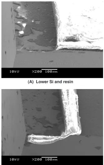
A crack ran brittly along an interface from the three- dimensional corner. Delamination surface was the interface between Si and resin. Photographs of SEM(Scanning Electron Microscope) of delamination surface in the specimen are shown in Fig.3. Figure 3(A) represents the debonding surface of lower Si and resin specimen, and Fig.3(B) represents the fracture surface of upper Si. The pictures show that the delamination occured at the interface between the upper Si and the resin. Through the precise observasion of the fracture surface, it was found that the delamination initiated at the corner of the joint. Hence, we perform stress analyses at the corner of interface bonding the upper Si and resin edge.

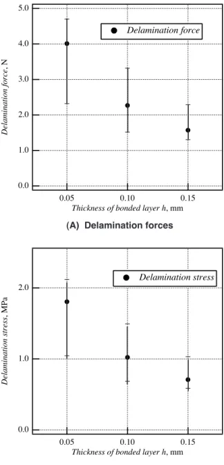
The results of the delamination test for each condition are shown in Fig.4. Delamination forces are shown in Fig.4(A), and stresses which are divided each load by bonding area

Test part load cell

Figure 1 Test specimen

(A) Testing apparatus

(B) Enlargement of test part

Figure 2 Schematic view of experimental apparatus 3.0

6.0

6.0

4.0

0.63

0.63 h F

Bonding area

Silicon Silicon Resin

A

0.37

Specimen Steel ball Jig 1

Jig 2

Figure 3 Fracture surfaces (A) Lower Si and resin

(B) The lower surface in the upper Si

Copyright © 2009 by ASME

are shown in Fig.4(B). Average forces for the thicknesses of resin of 0.05, 0.10 and 0.15mm are 4.01N, 2.27N and 1.57N, respectively. Average delamination stress is 1.81MPa for h=0.05mm, 1.02MPa for h =0.1mm and 0.71MPa for h=0.15mm. Hence, it is found that delamination force

decreased with increasing the thickness of resin. These experimental results are shown in Table 1.

ANALYSIS OF STRESS SINGULARITY Eigen analysis

In experiment, delaminatin occurs at the vertex of the interface between Si and the upper surface of resin, so eigen analysis at the vertex in a model for the specimen is performed. A model for eigen analysis is shown in Fig.5, where angles around the stress singularity point O are f

₁

=90º, f

₂

=180º, those around stress singularity lines are f

₁

=180º, f

₂

=180º at O

1

and f

₁

=180º, f

₂

=360º at O

2

.

Firstly, the order of stress singularity is determined using Eq.(3). The mesh division for eigen analysis is shown in Fig.6.

This figure represents a developed mesh on the q - f plane of the sphere surface shown in Fig.5. In this analysis, mesh size of q and f coordinates is q × f =15º×15º and a mesh involving an interface and stress singularity lines is equally divided by five. Material properties used in the analysis are shown in Table 2.

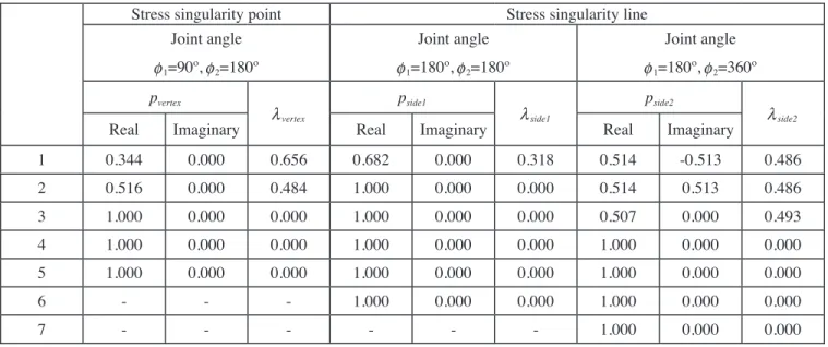
Results of eigen analysis are shown in Table 3. It is found that there are several eigen values yielding stress singularity

Material Young's modulus, GPa

Poisson's ratio

Thermal expansion, 10

^-6

/K

Silicon 169.1 0.26 3.0

Resin 2.97 0.38 33.0

Table 2 Material properties for analysis Resin Stress singularity

point upper surface of resin

θ _r φ φ

Silicon

O

2

φ

₁

Stress singularity line side1

side2

O₁ O2

Figure 5 Spherical coordinate system with an origin at a vertex

Figure 6 A mesh of the developed q× f plane(180º×360º model)

0 π/2

π/2

π

π

θ

2π φ

Interface Table 1 List of experimental results

number The bonded of layer

Thickness of resin,

mm

Adhesive area, mm

²

Average delamination

force, N

Average delamination

stress, MPa

1 0.05 2.22 4.01 1.81

2 0.10 2.22 2.27 1.02

3 0.15 2.22 1.57 0.71

(A) Delamination forces

(B) Delamination stresses

Figure 4 The comparison of experimental results 5.0

4.0 3.0 2.0 1.0 0.0

Delamination force , N

0.15 0.10

0.05 Thickness of bonded layer h, mm Delamination force

2.0

1.0

0.0

Delamination stress , MPa

0.15 0.10

0.05 Thickness of bonded layer h, mm Delamination stress

Copyright © 2009 by ASME

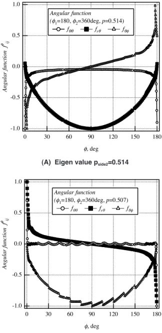
Figure 7 Distribution of angular function on the interface( f

1

=90º, f

2

=180º)

in each pair of the angle of vertexes in domains for analysis.

In the previous study[15] on the three-dimensional stress singularity, when a triple root of p=1 exists, logarithmic singularity occurs at the stress field. Then, the stress field at the vertex in three-dimensional joints can be expressed as follows.

σ

_ij

θ φ

_{kij kij}

θ φ

^λ

k M

k

r K f r

K

vertex

( , , ) ,

( )

= ( )

+

−

+

∑

1iij k ij lij lij

l l k

f

₍ +₎

( , ) K f , ln r

−

= +

+ ( ) ( )

1

2 2

θ φ ∑

^NN

θ φ ⁽⁸⁾

where r=r/h, N=M+3(with a triple root of p=1), N=M+4(with a quadruple root of p=1) when M is the number of l yielding stress singularity. l

vertex

represents the order of stress singularity at the vertex. Here, angular function f

ij

( q,f ) can be obtained from eigen displacement vector({u} on Eq.(3)) corresponding to eigen value p.

Angular functions at the interface for each eigen value of p

vertex

=0.344 and 0.516 in the joint angle f

₁

_=90º, f

₂

_{=180º is}

6.0 5.0 4.0 3.0 2.0 1.0 0.0

Angular function f

75 60 45 30

15 , deg

Angular function (

₁

=90,

₂

=180deg) f { =0.66 (p=0.344)}

f { =0.48 (p=0.516)}

Curve fitting

shown in Fig.7. In particular, the distribution of f

qq

( p /2, f ) relating to delamination at the interface is investigated. Here, f

qq

( p /2, f ) is expressed as f

qqf

( f ). The angular functions are normalized by the stress at f =60º. It is found from this figure that the angular function for p

vertex

=0.516 indicates the occurrence of singularity at only f =90º, so this angular function is not used for expressing the stress distributions in the present loading conditions. Hence, the order of stress singularity at the vertex with angles of f

₁

=90º, f

₂

=180º is l

_vertex

=0.66.

Angular functions for stress singularity lines are investigated using models of f

₁

=180º, f

₂

=180º and f

₁

=180º, f

₂

=360º. The order of stress singularity for stress singular line of f

1

=180º, f

2

=180º at O

1

is l

side1

=0.32 as shown in Table 3. Two eigen values exist in a model of f

1

=180º, f

2

=360º.

Angular functions f

ijf

( f ) for each eigen value p

side2

=0.514 and 0.507 are shown in Figs.8(A) and (B). In the present loading conditions, it is considered that s

qq

, s

_rq

are a symmetric and s

qf

is an odd functions with respect to f =90º. Hence, an angular function for p

side2

=0.507 is excluded from the expression for the stress distribution. Therefore, the order of stress singularity for stress singularity line of f

1

=180º, f

2

=360º is l

side2

=0.49.

The joint shape yielding the largest value of the order of stress singularity is the joint of angle f

₁

=90º, f

₂

=180º. Therfore, it would appear that delamination occurs the corner of jointed edge. The result may show that the observation on the delamination surface is valid.

Angular function f

qqf

( f ) in the singular stress field can be expressed as follows[16].

f

m side side

L

m side

side φθθ

θθ λ

ρ ρ φ ρ

(

1

,

2

, )

^{( )}1 1

=

^{− sside}1

L

^side

L L

m side side

m k

1 2

1 2

2

2

+

+ +

θθ −λ

θθ

( )

ρ

( ) ^{( )m side}θθθ

ln ρ

^{( )}θθ

k side

k

km side

k

L

1 3 6

1

2 2

=

∑ ( )

−

⁺

==

∑ ( )

− 3

6

2

lnρ

_side ^k 2

⁽⁹⁾

where r

_side1

_, r

_side2

are the distances from the point P( r _, q _, f _{) to} each stress singularity line in a spherical coordinate system, and they are expressed as r

side1

= r (1-sin

²

q cos

²

f )

^1/2

, r

side2

= r (1- sin

²

q sin

²

f )

^1/2

. Here, r is taken to 1. As remarked above, the Table 3 List of eigen values and the order of stress singularity for joints

Stress singularity point Stress singularity line

Joint angle f

₁

=90º, f

₂

=180º

Joint angle f

₁

=180º, f

₂

=180º

Joint angle f

₁

=180º, f

₂

=360º p

vertex

l

_vertex

^p

^side1

l

_side1

^p

^side2

l

_side2

Real Imaginary Real Imaginary Real Imaginary

1 0.344 0.000 0.656 0.682 0.000 0.318 0.514 -0.513 0.486

2 0.516 0.000 0.484 1.000 0.000 0.000 0.514 0.513 0.486

3 1.000 0.000 0.000 1.000 0.000 0.000 0.507 0.000 0.493

4 1.000 0.000 0.000 1.000 0.000 0.000 1.000 0.000 0.000

5 1.000 0.000 0.000 1.000 0.000 0.000 1.000 0.000 0.000

6 - - - 1.000 0.000 0.000 1.000 0.000 0.000

7 - - - - - - 1.000 0.000 0.000

Copyright © 2009 by ASME

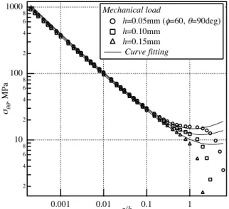
Figure 9 Distribution of stress, s

qq

, for external force against f on the interface(r/h=0.001, q =90º) 4x10

²

5 6 7 8 9

, MPa

90 75 60 45 30 15

0 , deg

Mechanical load

h=0.05mm, r/h=0.001, =90deg

h=0.10mm h=0.15mm

order of stress singularity of l

side1

=0.32 and l

side2

=0.49 are used for expressing the stress distribution in the singular stress region. The coefficients determined by approximating the angular functions by Eq.(9) are shown in Table 4.

Stress distribution in the singularity fields for mechanical loadings

Stress analysis using BEM is performed to determine the intensity of singularity at the vertex in the specimen shown in Fig.1. Domain method is employed in the BEM analysis.

Boundary condition is set as the same as delamination test, and an unit normal force to the specimen is applied on a point(see Fig.1). Eight nodes quadrilateral serendipity element is used, and the minimum length of side in an element near the vertex is 0.01 m m×0.01 m m. In this analysis, the thickness of resin is varied as 0.05mm, 0.10mm, 0.15mm. Material properties used in the analysis are shown in Table 2.

All stress components are transformed from a Cartesian coordinate system to a spherical coordinate system. Here, the results of analysis for mechanical loadings will be presented for several thicknesses in resin.

Distribution of stress, s

qq

, at a dimensionless distance, r/

h=0.001 on the interface( q =90º) against f is shown in Fig.9.

It is found that the stress, s

qq

, decreases with increasing the thickness of resin. Figure 10 shows a stress distribution normalized by the value of s

qq

at the angle f =60º occurring the minimum value in thermal residual stress analysis shown in the next section. It is found that all distributions are overlapped with each other. Stress distribution against angle f can be expressed as follows.

f

mBEM

H

side side BEM side

φθθ

ρ ρ φ

θθ

ρ

( )

(

1

,

2

, ) =

1( ) 1 _sside^side

H

^{BEM side} _side^side

H

1 1 2

1 22

−

+

−

+

λ ⁽θθ ⁾

ρ

λ

22 1

3 6

1 2

θθ θθ

ρ

(^BEM) k(BEM side)

ln

k side

H

k

+ ( )

+

=

∑

−

HH

kBEM side

k side

k

θθ

ρ

( ) ²

ln

3 6

2 2

=

∑ ( )

−

⁽¹⁰⁾

The coefficients determined by approximating the distribution of Fig.10 by Eq.(10) are shown in Table 5. H

1qq^(BEM)

is the intensity of singularity relating to the stress singularity line.

H

1qq^(BEM)

for the mechanical loading is represented by H

1qq^(M)

. External force affects little on the stress distribution varying the thickness of resin. The intensity of singularity at the side of f _{=0º, H}

_1qq^(M)side1

, is larger than that at the other side, H

1qq^(M)side2

.

Stress distribution on the interface against r/h at f =60º is Table 4 Coefficients in angular functions

l= _0.66 ^L

^1qq

(1)side1

L

1qq^(1)side2

L

2qq⁽¹⁾

L

3qq^(1)side1

L

3qq^(1)side2

1.325 0.375 -0.846 -0.102 0.022

l= 0.48 L

1qq^(2)side1

L

1qq^(2)side2

L

2qq⁽²⁾

L

3qq^(2)side1

L

3qq^(2)side2

0.087 0.834 -0.338 0.054 -0.042

(A) Eigen value p

side2

=0.514

(B) Eigen value p

side2

=0.507

Figure 8 Distribution of angular function on the interface( f

1

=180º, f

2

=360º)

-1.0 -0.5 0.0 0.5 1.0

Angular function f

ij

180 150 120 90 60 30 0

deg Angular function

(

₁

=180,

₂

=360deg, p=0.514) f f

_r

f

-1.0 -0.5 0.0 0.5 1.0

Angular function f

ij

180 150 120 90 60 30 0

deg Angular function

(

₁

=180,

₂

=360deg, p=0.507) f f

r

f

Copyright © 2009 by ASME

Figure 12 Model for thermal residual stress analysis x

x y

y z z

Fix in the x,y,z-directionFix in the y-direction Fix in the

y,z-direction

shown in Fig.11. The plots in this figure are almost overlapped.

The expression of stress distribution derived from Eq.(8) can be rewritten as follows.

σ

_θθ^BEM

r π φ

^BEM_θθ ^φ_θθ^BEM

h K f r

( , , ) 2

^{1 1( )}

h

= 

0

 



−..

( )

( )

ln

66

2 2

3 3

+

+

K f

K f r

BEM BEM

BEM BEM

θθ φθθ

θθ φθθ

hh K f r

BEM BEM

h

  

 + 

 



 



 

4 4



2

θθ φθθ( )

ln ⁽¹¹⁾

where the angular function calculated from Eq.(10), f

qqf

( f ), is normalized using the value at f =60º. The coefficients determined by a least square method using Eq.(11) are shown in Table 6. K

1qq^BEM

is the intensity of stress singularity with respect to the radial direction from the vertex O. K

1qq^BEM

for mechanical loadings is represented by K

1qq^Mech

. It is found that the value of intensity of singularity, K

1qq^Mech

, decreases with increasing the thickness of resin.

Stress distribution in the singularity fields for thermal loadings

Stress analysis for residual thermal stress is carried out by applying the tractions shown in Eq.(6) to the side surfaces of the specimen and by subtracting the tractions from a stress distribution after the calculation. Model for analysis is shown in Fig.12. Arrows are expressed the direction of external force.

Material property of Si does not vary with temperature, but resin varies. In this analysis, a variation of temperature from 298K to 423K is divided into 8 ranges, and BEM analysis is performed using a specified material property for each temperature range. The results of each range are summed up finally to obtain the stress distribution at room temperature.

Material property of Si is shown in Table 2. Material properties of resin for each temperature range are shown in Table 7. The order of stress singularity at the vertex varies due to a variation

Table 5 Determined coefficients in Eq.(10) for mechanical loadings

h, mm

Area,

mm

²

H

1qq^(M)side1

H

1qq^(M)side2

H

2qq^(M)

H

3qq^(M)side1

H

3qq^(M)side2

0.05 2.22 0.812 0.513 -0.629 -0.010 -0.059 0.10 2.22 0.832 0.509 -0.619 0.014 -0.042 0.15 2.22 0.836 0.493 -0.610 0.002 -0.055

Table 6 Determined coefficients in Eq.(11) for mechanical loadings

h, mm

Area,

mm

²

K

1qq^Mech

K

2qq^Mech

K

3qq^Mech

K

4qq^Mech

0.05 2.22 3.579 11.312 1.549 1.183 0.10 2.22 3.467 9.139 0.335 0.955 0.15 2.22 3.312 6.942 -0.782 0.732

Figure 11 Distribution of stress, s

qq

, for external force against r/h on the interface(f=60º, q=90º)

2 4 6

10

8 2 4 68

100

2 4 6

1000

8

, MPa

0.001 0.01 r/h 0.1 1

Mechanical load

h=0.05mm ( =60, =90deg) h=0.10mm

h=0.15mm Curve fitting

Figure 10 Distribution of normalized stress, s

qq

, for external force against f on the interface(r/h=0.001, q =90º)

1

2

Normalized stress

90 75 60 45 30 15

0 deg

Mechanical load

h=0.05mm, r/h=0.001, =90deg h=0.10mm

h=0.15mm Curve fitting

Copyright © 2009 by ASME

Table 8 Determined coefficients in Eq.(10) for thermal loadings

Table 9 Determined coefficients in Eq.(11) for thermal loadings

h, mm Area,

mm

²

K

1qq^Ther

K

2qq^Ther

K

3qq^Ther

K

4qq^Ther

0.05 2.22 6.374 -39.620 17.612 2.696 0.10 2.22 7.165 -17.719 24.469 3.624 0.15 2.22 7.591 -11.436 26.044 3.997 h,

mm Area,

mm

²

H

1qq^(T)side1

H

1qq^(T)side2

H

2qq^(T)

H

3qq^(T)side1

H

3qq^(T)side2

0.05 2.22 1.434 0.294 -0.933 -0.052 -0.029 0.10 2.22 1.273 0.343 -0.840 -0.036 -0.040 0.15 2.22 1.174 0.362 -0.771 -0.034 -0.050 Figure 15 Distribution of thermal residual stress, s

qq

,

against r/h on the interface(f=60º, q =90º) 1

10 100 1000

, MPa

2 3 4 5 6 7

0.001

²

r/h

^{3 4 5 6 7}

0.01

^{2 3 4 5}

h=0.025mm, =60, =90deg

h=0.05mm h=0.075mm

h=0.1mm h=0.15mm

Curve fitting of material property with temperature. The order of stress

singularity also listed in Table 7. It is found that the order of stress singularity at a higher temperature is larger than that at a lower temperature. In this analysis, two digit of the average value of the order of stress singularity is used for expressing the stress distribution of residual thermal stress.

The results of analysis for thermal loadings are shown for various values of the thickness of resin. The thickness of resin is varied as 0.025mm, 0.05mm, 0.075mm, 0.10mm, 0.15mm.

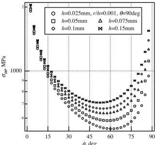
Distribution of stress, s

qq,

against f at r/h=0.001 on the interface is shown in Fig.13. Normalized stress using the value of s

qq

at f =60º is shown in Fig.14. It is found that the value of stress decreases with increasing the thickness of resin, and a relationship between the thickness of resin and the normalized stress reverses at f =60º. The distribution for normalized stress is approximated by Eq.(10) as the case of mechanical loadings, the coefficients are determined using a least square method, and their values are shown in Table 8. H

1qq^(BEM)

for thermal

Figure 14 Distribution of normalized thermal residual stress, s

qq

, against f on the interface(r/h=0.001, q=90º)

1

2 3

Normalized stress

90 75 60 45 30 15

0 , deg

h=0.025mm, r/h=0.001, =90deg h=0.05mm h=0.075mm h=0.1mm h=0.15mm Curve fitting

Table 7 Material property of resin Temperature Young's

modulus

Thermal expansion

Poisson's ratio

The order of stress singularity T, K D T, K E, GPa a _{, 10}

^-6

_/K n l

298-314 16 2.86 33 0.38 0.656 0.484

314-330 16 2.66 33 0.38 0.658 0.486

330-346 16 2.57 33 0.38 0.658 0.487

346-362 16 2.37 33 0.38 0.659 0.488

362-378 16 2.11 33 0.38 0.661 0.490

378-393 15 1.96 40 0.38 0.662 0.491

393-408 15 1.56 66 0.38 0.665 0.494

408-423 15 0.78 86 0.38 0.670 0.501

Average - - - - 0.661 0.490

6 7 8 9

1000

2

, MPa

90 75 60 45 30 15

0 , deg

h=0.025mm, r/h=0.001, =90deg h=0.05mm h=0.075mm h=0.1mm h=0.15mm

Figure 13 Distribution of thermal residual stress, s

_qq

, against f on the interface(r/h=0.001, q =90º)

Copyright © 2009 by ASME

Table 10 Determined coefficients in Eq.(10) for superposed stress distribution

Table 11 Determined coefficients in Eq.(11) for superposed stress distribution

h, mm

Area,

mm

²

K

1qq^M+T

K

2qq^M+T

K

3qq^M+T

K

4qq^M+T

K

5qq^M+T

0.05 2.22 7.654 29.307 -8.839 -4.935 -1.177 0.10 2.22 4.570 14.642 -1.221 -2.960 -0.783 0.15 2.22 3.139 9.192 0.101 -1.887 -0.490 h,

mm Area,

mm

²

H

1qq^(M+T)side1

H

1qq^(M+T)side2

H

2qq^(M+T)

H

3qq^(M+T)side1

H

3qq^(M+T)side2

0.05 2.22 0.873 0.312 -0.480 -0.076 -0.169 0.10 2.22 0.895 0.308 -0.492 -0.090 -0.159 0.15 2.22 0.829 0.283 -0.408 -0.134 -0.178

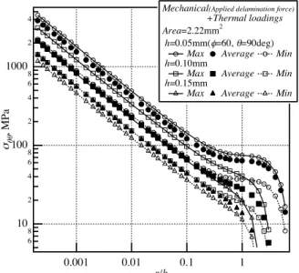
Figure 18 Superposed stress distribution, s

qq

, against r/h on the interface

10

2 3 45 6

100

2 3 45 6

1000

2 3 4

, MPa

0.001 0.01 0.1 1

r/h

Mechanical(Applied average delamination force) +Thermal loadings Area=2.22mm²

h=0.05mm ( =90, =60deg) h=0.10mm h=0.15mm Curve fitting

Figure 17 Superposed stress distribution, s

qq

, against f on the interface

1

2

Normalized stress

90 75 60 45 30 15

0 , deg

Mechanical

(Applied average delamination force)

+Thermal loadings Area=2.22mm

²

h=0.05mm (r/h=0.001, =90 deg) h=0.10mm h=0.15mm loadings is represented by H

1qq^(T)

. It is found that the intensity

of singularity relating to the stress singularity line is not so much varied with the thickness of resin, and an intensity of singularity near the free side surface, H

1qq^(T)side1

, is larger than that near the other side, H

1qq^(T)side2

. The distribution of stress, s

qq,

against r/h at f =60º on the interface is shown in Fig.15.

This distribution is approximated by Eq.(11) as the case of mechanical loadings, and the coefficients are determined. Their values are shown in Table 9. K

1qq^BEM

for thermal loadings is represented by K

1qq^Ther

. It is found that the intensity of singularity in the radial direction increases with increasing the thickness of resin.

Stress distribution at the singular stress region Stress distribution at delamination in the singular stress field is obtained by superposing the stress fields for mechanical and thermal loadings. Here, a stress distribution for a critical stress condition is calculated multiplying the stress field for mechanical loading by a delamination force. Stress distributions at the maximum, the minimum and the average forces for delamination are shown in Fig.16. It is found that a data scatter exists in experiment, however, larger stress is needed to delaminate in the joint with a thinner resin layer.

Here, the strength of interface is evaluated using the average force for delamination.

Stress distribution for angle f in the singular stress field is shown in Fig.17 for several values of thickness of resin. In this figure, larger stress occurs near f =0º in the joint with a thicker resin layer, and a relationship between normalized stress and angle f reverses at f =60º. Stress distribution against r/h is shown in Fig.18 for several values of the thickness of resin.

The value of stress decreases with increasing the thickness of resin. These stress distributions are approximated by Eq.(10), (11), and the coefficients are determined. The values of coefficients are shown in Tables 10, 11. K

1qq^BEM

and H

1qq^(BEM)

for mechanical and thermal loadings are represented by K

1qq^M+T

and H

1qq^(M+T)

, respectively. It is found that K

1qq^M+T

decreases with

Figure 16 Distribution of stress, s

qq

, against r/h on the interface considering delamination force

68

10

2 4 68

100

2 4 68

1000

2 4

, MPa

0.001 0.01 0.1 1

r/h

Mechanical(Applied delamination force) +Thermal loadings Area=2.22mm²

h=0.05mm( =60, =90deg) Max Average Min h=0.10mm

Max Average Min h=0.15mm

Max Average Min

Copyright © 2009 by ASME

Figure 19 Determination of critical stress intensity factor for bonded joints against delamination force 2.5

2.0 1.5 1.0 0.5 0.0 K

3D critical

, MPa*m m

0.66

5.0 4.5 4.0 3.5 3.0 2.5 2.0 1.5 1.0 0.5

0.0 Delamination force, N h=0.05mm

h=0.10mm h=0.15mm increasing the thickness of resin, and H

1qq^(M+T)side1

is larger than

H

1qq^(M+T)side2

.

DISCUSSION

The intensity of singularity for both f and r directions is required for evaluating the strength of interface in three- dimensional joints. By substituting Eq.(10) into Eq.(11), the intensity of singularity at the vertex in the three-dimensional joints can be expressed as follows.

σ

_θθ^BEM

( r , ρ

_side1

, ρ

_side2

) ⁼ K

₁^BEM_θθ

H

₁⁽_θθ^{BEM sid) ee side}

BEM side

H

side

H

1 0 321

1 2

0 492

ρ

θθ

ρ

−

−

(

+ +

.

( ) .

22

0 66 2

θθ θθ

BEM

r K

BEM

( )

)

^−.

^{+ (12)}

Here, the logarithmic terms are neglected for simplicity.

Because, it was already shown in [13] that the logarithmic terms affect on the stress distribution far from the vertex, and the power law singularity represented by a line in the double logarithmic plot was dominant in this analysis.

Singular stress fields considering residual thermal stresses under a delamination condition can be expressed as follows.

σ

_θθ^Mech

( r , ρ

_side1

, ρ

_side2

) ⁺ σ

_θθ^Ther

r , ρ

_side1

, ρ

_s^iide

Mech M side

K F H

side

H

2

1 1 1

0 321

( )

=

^θθ

(

^{( )θθ}

^ρ

^−.

⁺

11 2 0 492

2 0 66

2

θθ θθ

θθ

( )M side

ρ

. .

side

H

M

r

K

−

+

( )

)

⁻

+

^MMech

+ K

^1Therθθ

( H

^{1( )θθT side1}

^ρ

_side^{−0 32.1}

⁺ H

^{1(( )θθT side side. T .}

The

H r K

2 0 492 2

0 66

2

ρ

_θθ

θθ

−

+

( )

)

⁻

+

^rr

₍₁₃₎

where F represents the force for delamination. Equation (13) is factorized by the term with a larger intensity of singularity.

Thus,

σ

_θθ^Mech

( r , ρ

_side1

, ρ

_side2

) ⁺ σ

_θθ^Ther

r , ρ

_side1

, ρ

_s^iide

Mech M side

K H

side

H

2

1 1 2

0 491 1

( )

=

_θθ ^{( )}_θθ

ρ

^{−. (( )}_{( )}^θθ_{M side}^{M side side.}_.

H

side

1 0 322

1 2

0 491

ρ

θθ

ρ

−

−

++ +









 



^{( )}

1

² −

1 2

0 491

H H

M M side

side θθ

θθ

ρ

( ) .





 



+

⁻

F

K H

Ther T side

H

side

1 1 2

0 491 1

θθ ^{( )}θθ

ρ

^. θ^θθ

θθ

ρ ρ

( ) .

( ) .

T side T side side

H

side

1 0 322

1 2

0 41

−

− 99 2

1 2

0 491

1

 + +







 

( )

H

−

H

T T side

side θθ

θθ

ρ

( ) .





+ ( ^K

2^Mech

+ ^K

2^Ther

) ^{r } _ ^r

⁻

0 66 0 66

θθ θθ

. .

(14)

Here,

φ → ρ →

→ →

90

−

1 0

0 0

0 491 0 66

then r then r

side. .

therefore,

σ

_θθ^Mech

( r , ρ

_side1

, ρ

_side2

) ⁺ σ

_θθ^Ther

r , ρ

_side1

, ρ

_s^iide

Mech M side Ther

K H F K H

2

1 1 2

1 1

( )

= (

_θθ ^{( )}_θθ

+

_θθ ^{(TT side}_θθ^{) 2}

) ^ρ

_side⁻0 49^.1

r

⁻0 66^.

⁽¹⁵⁾

Coefficients in (15) is used to evaluate the strength of interface in delamination test. Hence, a critical intensity of singularity is expressed as follows.

K

Dcritical

K

DMech

F K

DTher

h

13

13

13 0 6

θθ

= (

θθ

+

θθ

)

^{. 66}

⁽¹⁶⁾

where, K

1qq^3DMech

and K

1qq^3DTher

represent K

1^BEMqq

H

1qq^(BEM)side2

for mechanical and thermal loadings, respectively. A value

obtained from Eq. (16) includes the effect of thickness of resin on the critical intensity of singularity, K

1qq^3Dcritical

. Hence, the value of critical intensity of singularity is uniquely determined whatever the thickness of resin is.

Equation (16) against delamination force is drawn in Fig.19.

Fine lines indicate the intensity of singularity for delamination force in experiments. Generally, data of delamination in experiment scatter, however, it is found that their lines converge on about K

1qq^3Dcritical

=1.4MPa•mm

^0.66

. In the present study, it is estimated that the critical strength of interface is about K

1qq^3Dcritical

=1.4MPa•mm

^0.66

.

CONCLUSION

In the present paper, the strength of interface in three- dimensional joints with several values of the thickness of resin was analyzed considering residual thermal stresses using BEM and eigen analysis. The critical strength of interface was evaluated from singular stress fields considering residual stresses under a delamination condition. As a result, the following items could be obtained.

(1) Angular functions for several values of the order of stress singularity are derived from eigen analysis, and the expressions for stress distribution are determined comparing the angular functions and the stress distribution obtained from BEM. (2) An expression for the critical strength of interface is derived combining mechanical and thermal loadings. The critical strength of interface determined in the present study was about K

1qq^3Dcritical

=1.4MPa•mm

^0.66

.

REFERENCES

[1] Inoue, T. and Koguchi, H. 1996, "Influence of the

Intermediate Material on the Order of Stress Singularity in

Three-Phase Bonded Structure", Int. J. Solids Structures,

Vol.33, pp.399-417. Copyright © 2009 by ASME

[2] Qian, Z. Q. and Akisanya, A. R., 1999, "An Investigation of the Stress Singularity near the Free Edge of Scarf Joints", Eur.

J. Mech. A/Solids, Vol.18, pp.443-463.

[3] Reedy, JR. and Guess, T. R., 1997, "Interface corner failure analysis of joint strength: Effect of adherend stiffness", Int. J.

Fracture, Vol.88, pp.305-314.

[4] Koguchi, H. and Muramoto, T., 2000, "The Order of Stress Singularity near the Vertex in Three-Dimensional Joints", Int. J.

Solids Structures, Vol.37, pp.4737-4762.

[5] Labossiere, P. E. W. and Dunn, M. L., 2001, "Fracture Initiation at Three-Dimensional Bimaterial Interface Corners", J. Mech. Phys. Solids, Vol.49, pp.609-634.

[6] Bogy, D.B., 1970, "On the Problem of Edge-Bonded Elastic Quarter-Planes Loaded at the Boundary", Int. J. Solids Structures, Vol.6, pp.1287-1313.

[7] Bogy, D.B., 1971, "Two Edge-Bonded Elastic Wedges of Different Materials and Wedge Angles under Surface Tractions", J.Appl. Mech., Vol.38, pp.377-386.

[8] Bogy, D.B., 1971, "On the Plain Elastostatic Problem of a Loaded Crack Terminating at a Material Interface", J. Appl.

Mech. Vol.38, pp.911-918.

[9] Bogy, D.B. and Wang, K.C., 1971, "Stress Singularities at Interface Corners in Bonded Dissimilar Isotropic Elastic Materials", Int. J. Solids Structures, Vol.7, pp.993-1005.

[10] Dempsey, J.P. and Sinclair, G.B., 1979, "On the Stress Singularities in the Plane Elasticity of the Composite Wedge", J.

Elasticity, Vol.9, pp.373-391.

[11] Pageau, S. S. and Bigger, Jr S. B., 1995, "Finite Element Evaluation of Free-Edge Singular Stress Fields in Anisotropic Materials", Int. J. Numer. Methods Eng, Vol.38, pp.2225-2239.

[12] Yuuki, R.ed., 1993, "Mechanics of Interface", p.55, Baifuukan.

[13] Koguchi, H. and Meo, N., 2006, "An Evaluation of Interface Strength at a Vertex in a Three-Dimensional Joint Considering Residual Thermal Stresses Using Three Dimensional Boundary Element Method", Trans. Jpn. Soc.

Mech. Eng. Vol.72, No.723, pp.1598-1606.

[14] Koguchi, H. and Taniguchi, T., 2007, "Evaluation of Interface Strength at the 3D-Corner in Si-resin Considering Residual Thermal Stresses", The ASME 2007 InterPACK Conference, 33592, Vancouver, BC, CANADA, July-8-12.

[15] Monchai, P., and Koguchi, H., 2007, "Boundary Element Analysis of the Stress Field at the Singularity Lines in Three- Dimensional Bonded Joints under Thermal Loading", J.Mechanics of Materials and Structures, Vol.2, No.1, pp.149- 166. [16] Koguchi, H. and Taniguchi, T., 2008, "Characteristics of Stress Singularity Field of Residual Thermal Stresses at vertex in Three-Dimensional Bonded Joints", Trans. the Japan Soc.

Mech. Eng., Ser. A, Vol.74, No.724, pp.864-872.

Copyright © 2009 by ASME