Kyushu University Institutional Repository

九州大学学術情報リポジトリ

Kyushu University Institutional Repository

飛来物の高速衝突を受けるコンクリート版の衝撃貫 通挙動に関する解析的研究

路, 馳

http://hdl.handle.net/2324/4110413

出版情報：Kyushu University, 2020, 博士（工学）, 課程博士 バージョン：

権利関係：

An Analytical Study on the Penetrating Behavior of Concrete Slab Subjected to

High Velocity Projectiles

Lu Chi

2 0 2 0

Department of Civil and Structural Engineering

Graduate School of Engineering

Kyushu University

i

Index

Chapter 1 Introduction 1

1.1 Background 1

1.2 Related works 2

1.3 Objective and composition 3

1.3.1 Objective 3

1.3.2 Composition 3

Chapter 2 Theory of SPH 5

2.1 Concept of SPH 5

2.2 Formulation of SPH 7

2.2.1 Integral representation of functions 7

2.2.2 Integral representation of derivatives 9

2.2.3 Particle approximation 11

2.2.4 Formulation method of SPH 13

2.3 Kernel function 15

2.3.1 Conditions of kernel function 15

2.3.2 Typical example 17

2.4 Numerical aspects 19

2.4.1 Artificial viscosity 19

2.4.2 Smoothing length 21

2.4.3 Symmetry of interaction 22

Chapter 3 Application of SPH in numerical analysis 25

3.1 Analysis procedure of SPH method 25

3.2 Pariticle approximation 25

3.2.1 Basic theory and formula of ASPH method 25

ii

3.2.2 Kernel function used in this study 26

3.2.3 Smoothing length used in this study 27

3.3 Time integration 28

3.3.1 Numerical integration method 28

3.3.2 Time integration in this study 29

3.3.3 Stability of explicit methods 29

3.4 Calculation of acceleration, velocity, and displacement 29

3.5 Calculation of strain 31

3.6 Calculation of stress 32

3.7 Calculation of contact force 33

Chapter 4 Material constitutive law in impact analysis 35

4.1 Introduction 35

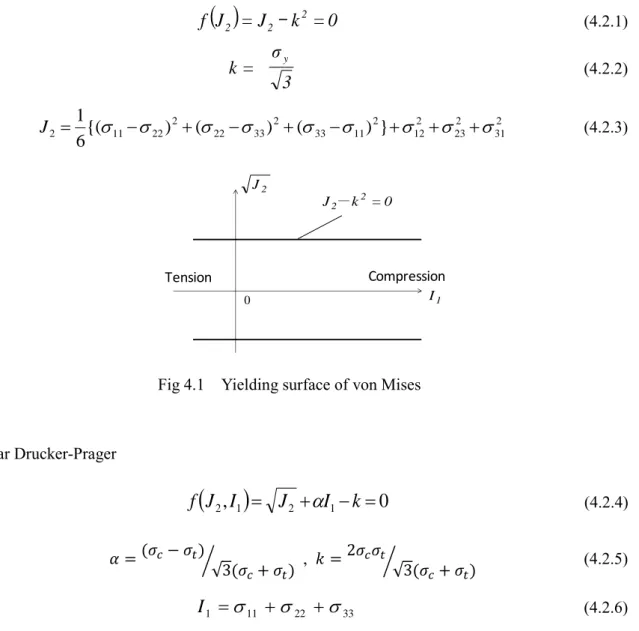
4.2 Yielding conditions of materials 35

4.3 Derivation of elastoplastic constitutive law 37

4.3.1 Derivation of stiffness matrix 37

4.3.2 Calculation of associated flow rules and plastic strain increments 44 4.3.3 Calculation of equivalent stress and equivalent plastic strain 47

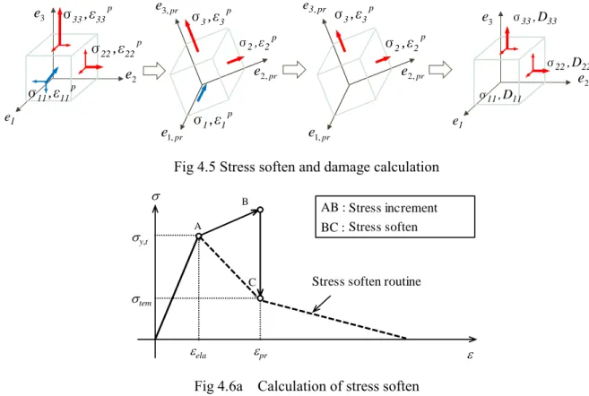
4.4 Softening behavior and damage of concrete materials 49

4.4.1 Tensile softening behavior and tensile damag e 49

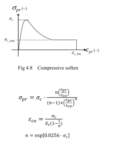
4.4.2 Compressive softening behavior and c ompression damage 53

4.5 Crushing 54

4.6 Strain rate effect 55

4.6.1 Calculation of Dynamic Increase Factor 56

4.6.2 Verification analysis of strain rate effect 57

Chapter 5 Verification analysis for the proposed SPH impact analysis method 61

5.1 Introduction 61

5.2 Validity verification of impact response analysis using RC beam 61

iii

5.2.1 Previous experimental models and analysis overview 61

5.2.2 Results and discussion 63

5.3 RC slab penetration analysis 64

5.3.1 Analysis objects 64

5.3.2 Results and discussion 66

5.4 Conclusion 69

Chapter 6 Discussion on penetration fracture by SPH method 71

6.1 Introduction 71

6.2 Analysis model and cases 71

6.3 Analysis of penetration failure 72

6.4 Effect of impact velocity on impact force and impulse 73

6.5 Discussion on the penetration failure of different impact velocity 75 6.6 Effect of the mass of the projectile on penetrating impulse 76 6.7 Effect of supporting condition of concrete slab on penetration impulse 77

6.7.1 Comparison between 4-side support and 2-side support 77

6.7.2 Relationship between supporting interval and impulse 78

6.8 Conclusion 79

Chapter 7 Proposal of evaluation method for penetration damage 81

7.1 Introduction 81

7.2 Penetration damage criterion equation based on impulse 81

7.2.1 Determination of the maximum impact force 82

7.2.2 Determination of the impact duration 84

7.2.3 Determination of the impulse criterion equation 85

7.3 Validity verification of the impulse equation 86

7.3.1 Verification of consistency between analysis response results and impulse

equation 87

7.3.2 Comparison with other empirical equations 88

iv

7.4 Conclusion 91

Chapter 8 Conclusion 93

8.1 Key conclusions and achievements 93

8.2 Future works 94

Reference 95

Acknowledgments 100

1

Chapter 1 Introduction

1.1 background

In recent years, to prevent serious damage from natural disasters such as tornados and volcanic eruptions, the demand for protecting structures against the collision of flying objects is recognized in Japan, and it is important to predict the impact performance (penetration prevention) of these structures.

Not only in Japan, the damage done by natural disasters are not a rare case in many oversea countries.

U.S. Nuclear Regulatory Commission has already established design code considering the collision of flying objects towards nuclear facilities¹⁾. As a container for nuclear fuels and structures protecting the security system for the nuclear plant, the durability against such disasters is required. On the other hand, to give an example for volcano eruption, the Mt. Ontake erupted on September 27th, 2014. Car accidents were caused by the high-velocity rocks erupted, which raised focus on the necessity of rock sheds. Along with these natural disasters such as tornados and volcano eruptions, structures and sheds are collided with high-velocity rocks and other projectiles, resulting in severe damage. Fig 1.1 shows many damage pattern caused by high-velocity projectiles, and researches aiming the impact phenomena has already started in the 1930s. From these researches, it is also known that there is a possibility of secondary disaster after the primary damage.

(a) surface damage (b) spalling (c) perforation Fig 1.1 damage pattern of concrete slab

2

Generally, for the slight plastic deformation of structures, it is confirmed that the prediction can be easily done by universal FEM software. While for the large deformation relating to high-velocity projectiles and penetrations, the prediction is difficult to be conducted, the accuracy of the analysis result is not yet validated, and the demand for the complex design of the structures against such penetration and local damage is growing. On the other hand, the experimental research conducting on the RC slabs for the evaluation of penetration performance consumes lots of time to prepare, and faces the financial problem constraining the actual experiment scales and trial numbers. Based on the given background, it is important to build up a meshless analytical method evaluating the penetration performance of RC concrete slabs.

1.2 Related works

In order to comprehend the current research progress relating to the impact response analysis of the structures in Japan and other countries, here we summarized the researches relating to the penetration and local damage experiments conducted on concrete, the empirical formula, and the analytical researches.

For the existing studies on the local failure prevention measure, Beppu et al. ²⁾ performed collision with a mushroom-shaped projectile on concrete plates. Kojima³⁾ conducted a set of tests with various RC slab targets and projectiles, inferring that the local damage of RC slab is the most related to the hardness of projectile’s nose and more reinforcement would reduce local damage against hard-nose projectile. M.H Zhang et al. ⁴⁾ pointed out that the perforation depth and crater diameter of high-strength concrete due to collision can be reduced by the increase of compressive strength and the presence of coarse granite aggregates.

Formulae have been developed based on experimental results, to predict the perforation depth and the critical slab thickness for perforation and scabbing of reinforced concrete to occur. Kennedy⁵⁾ compared and reviewed formulae of modified Petry, ACE (Army Corps of Engineers), BRL (Ballistic Research Laboratory), modified NDRC (National Defense Research Committee) and Ammann and Whitney and the Ballistic Research Laboratory. There are also formulae proposed by Hughes⁶⁾ to evaluate the perforation depth, critical slab thickness for scabbing, and critical slab thickness against perforation.

3

For existing studies, the perforation limit of a concrete slab has been examined by experiments, while impact tests were usually performed by small scale specimens due to the limitation of experimental conditions. Furthermore, it is still difficult to predict the accurate local failure of the concrete structure.

The use of numerical analysis is a powerful alternative to study impact phenomena in term of scale and cost. In general, FEM is not suitable to simulate the discontinuous displacement field such as perforation process. Therefore, Smoothed Particle Hydrodynamics (SPH) as one of the particle methods that can reproduce local failure of concrete structural members such as crushing or perforation is utilized. SPH is a particle-based Lagrangian method for solving systems of partial differential equations.

SPH was originally invented for astrophysical applications^7,8). Since its invention, it has been successfully applied to a vast range of problems such as the dynamic response of material strength^9,10), fluid flow¹¹⁾, etc.

1.3 Objective and composition

1.3.1 Objective

In this study, based on the given background, SPH method, which is one of the meshless analytical methods and suitable for problems relating to the large deformation and damage of solid body, is adopted. Then a mechanical model for the penetration phenomenon is built, and the results of the experiment and the SPH analysis is compared to validate the proposed analysis method. By using the proposed analysis method, the influence of different projectile and impact velocity on the penetration response of concrete slab and the impulse consumed is investigated. Finally, an evaluation method for the penetration/perforation damage of the concrete slab based on the impulse calculation is proposed.

1.3.2 Composition

This paper is composed of 8 chapters. The outline of each chapter is described below.

In Chapter 1, Introduction, the background and purpose of this study, and the previous studies, the importance and problems of performance evaluation for penetration prevention are described, and the structure of this paper is shown.

In Chapter 2, Theory of SPH Method, the basic concept of SPH (Smoothed Particle Hydrodynamics) method is explained, which is the main analysis method of this research.

4

In Chapter 3, Application of SPH in numerical analysis, the procedure of analysis using SPH method in this study is described, and the contact algorithm is also described.

In Chapter 4, Material constitutive law in impact analysis, a mechanical model of concrete material used for impact analysis with penetration is described.

In Chapter 5, Verification analysis for the proposed SPH impact analysis method, the validity and the accuracy of the proposed SPH analysis method is verified by comparing analysis results with a falling weight experiment on RC beam and a perforation experiment on concrete slab.

In Chapter 6, Discussion on penetration fracture by SPH method, a concrete slab is taken as the analysis object, and the damage of the projectile done to this concrete slab is discussed based on numerical analysis results.

In Chapter 7, Proposal of evaluation method of penetration damage, an impulse equation is established to predicted the consumed impulse of the projectile during penetration process.

In Chapter 8, Conclusions, the results obtained in this study are summarized and the tasks needed in the future are described.

5

Chapter 2 Theory of SPH

The SPH method was proposed by Lucy and Monaghan et al. In the late 1970s^1,2), and is an analysis method based on particle representation based on the compressed fluid theory. Basically, hydrodynamic problems are solved in the form of differential equations of the deviation of variables such as density, velocity, energy, etc. Since then, it has been extensively studied and applied to astrophysical problems in three-dimensional space, dynamic response including material strength, and impact analysis of solids with large deformation. In this chapter, the SPH method will be described first, followed by a description of the SPH method applied to general solid problems.

2.1 Concept of SPH

The SPH method is a particle-based mesh-free method, and, like other mesh-free particles, the computational framework is not a grid cell in the finite difference method nor a mesh element in the finite element method, but particles in a 3D space with no need to pre-define connectivity between them.

In SPH, the particle approximation described in Section 2.2 is performed for particles in the smoothing length at each time step. However, since it is almost impossible to solve a set of partial differential equations analytically except in very rare cases, as the solution procedure, the problem domain defined by the partial differential equations is first discretized, then method to approximate the region function and its derivative value at random point is needed. Therefore, approximate equations are applied to partial differential equations to create discretized ordinary differential equations that depend only on time increment. This discretized ordinary differential equation can be solved using time integration such as the finite difference method. In order to execute such a solution, the SPH method is performed as follows.

1. First, the problem area is represented by arbitrarily distributed particles. There is no need for binding to these particles. (Mesh free)

2. An integral representation is used to approximate the domain function. This is called kernel approximation in the SPH method. (Integration function display)

6

3. The kernel approximation is performed using particles. This is called particle approximation in SPH, which is to replace the integral representation of the region function and its derivative with the sum of all the corresponding values of the particles within the local region called the supporting domain. (Compact support)

4. Since particle approximation is performed at each time step, the use of particles depends on the local distribution of particles. (Adaptation)

5. Particle approximation is performed on all terms related to the domain function of the partial differential equation to create a discretized ODE that depends only on time. (Lagrange)

6. Ordinary differential equations are solved using explicit integration to speed up calculations and obtain time history of field variables for all particles. (Dynamic)

Step 1 stipulates the mesh-free properties of the SPH method. It is not difficult to formulate a numerical method without using a mesh, but when Neumann boundary conditions are used for irregular nodes and particles in the region, it is important to ensure the stability of the numerical method.

Step 2 provides the stability necessary for the SPH method mathematically because the integral representation is a weak form with smoothing effect. As long as the numerical integration is done correctly, the weak form is often very stable.

Step 3 creates discretized banded and sparse matrices. Problems with large deformations require a large number of particles to represent the problem area, and it takes a very long time to solve a huge amount of equations. At this point of view, this is a very important point in terms of computational effects.

By performing Step 4, SPH adaptability can be obtained at each time step based on any particles distributed within the smoothing length. Since this adaptable SPH approximation is performed early in the field variable approximation, the SPH formulation is not affected by any time-varying particle partitioning and therefore can handle very large deformation problems. It should be noted that this particle approximation is a method of numerical integration required for Step 2. Also, enough particles must be used to guarantee the accuracy and numerical stability of the integration.

In Step 5, the use of Lagrange will give the SPH method all the features of the Lagrange method.

Step 6 is the standard time integral methods for solving dynamic problems. What the SPH method should do is to determine an appropriate method for determining the time step to guarantee a stable

7 time integration.

Thus, these six steps guarantee the SPH method as mesh-free, adaptability, stability, and Lagrangian solutions to dynamic problems.

The SPH method can be applied from very small scales to very large scales, from astrophysics to fluid and solid mechanics problems, as well as very irregular and uniform dynamic shape problems. It is believed that deformation problems and impact problems can be easily dealt with. SPH can sometimes be affected by numerical problems such as inaccurate boundaries and tension instability, which can lead to large errors in these situations, but the accuracy can be improved by various corrections. Thus it can be said that SPH is a very versatile method.

2.2 Formulation of SPH

The SPH approximation includes continuous integral representation (kernel approximation) and arbitrary particle approximation, which are the principles of the SPH method. Since this involves complex partial differential equations, the SPH formulation can be divided into two stages. The first step is an integral representation of the field function, or kernel approximation, and the second step is particle approximation. Here we explain these two stages.

2.2.1 Integral representation of functions

In the first step, the integral of the product of the arbitrary function and the kernel function gives a kernel approximation to the integral representation of the function. The integral representation of the function can be approximated by summing the values at the interpolation points. This gives a particle approximation of the function with discrete points and particles. The concept of integral representation of the function f(x) used in the SPH method is expressed by equation (2.2.1).

' ) ' ( ) ' ( )

(x f x x x dx

f











(2.2.1)

Here f is the function of position vector x, and (xx') is Dirac delta function, with definitions shown below





 

 



 x x

x x x

x 0

) 1 '



( (2.2.2)

In equation (2.2.1),  is the integration range including x. Equation (2.2.1) means that the function

8

can be expressed in the form of an integral. Since the Dirac delta function is used, as long as f (x) is defined continuously in  , the integral representation of Equation (2.2.1) holds. If delta function

) ' (xx

 is replaced with the kernel function W(xx',h) , the integral representation of (2.2.1) is given by

' ) , ' ( ) ' ( )

(x f x W x x h dx

f







 (2.2.3)

Here, h is the smoothing length defined as the influence range of the kernel function W. As long as W is not a Dirac function, the integral representation of (2.2.3) can only be an approximation. This is the starting point of the kernel approximation. Equation (2.2.3) may be expressed as the following equation (2.2.4).

' ) , ' ( ) ' ( )

(x f x W x x h dx

f







 (2.2.4)

The kernel function W is generally an even function, but there are some conditions that must be met³⁾. The first condition is that it is standardized.







 ', ) ' 1 (x x h dx

W (2.2.5)

This condition is called the unity condition because it is the integral of the kernel function that produces 1. The second condition is the characteristic of the delta function can be found when the smoothing length approaches zero.

W



x x h

 

x x



h

 

 

  ,



lim

0 (2.2.6)

The third condition is compact condition

W(xx',h)0 when xx' 



h (2.2.7) where  has a certain relationship with the kernel function at the point x and is defined as a valid (non-zero) region of the kernel function. This effective region is called the support domain of the kernel function at point x. Also, by using the compact condition, the integration in the problem domain concentrates on the integration in the support domain of the kernel function. Therefore, the integration region  can be treated in the same way as the support domain. Equation (2.2.7) shows that the support domain of the kernel function is xx' 



h.

9

The error of SPH integral representation can be estimated by using the Taylor series expansion of the function around the point. Here f (x) is a differentiable function. From equation (2.2.4)

 

) ( ' ) , ' ( ) ' ( ) ( ' ' ) , ' ( ) (

' ) , ' ( ) ) ' ((

) ' )(

( ' ) ( )

(

2 2





































h r dx h x x W x x x f dx h x x W x f

dx h x x W x x r x x x f x f x

f

　　 ^(2.2.8)

where r means the remainder. Since W is an even function depending on x, (x'x)W(xx',h) becomes an odd function. Therefore, the following equation (2.2.9) holds.



 

 

 ,



0



 x x W x x h dx (2.2.9)

Substituting Equation (2.2.5) and Equation (2.2.9) into Equation (2.2.8) )

( ) ( )

(x f x r h²

f   (2.2.10)

From the above equation, it can be seen that the SPH method has second-order accuracy for the integral representation of the function and the kernel approximation. However, the kernel approximation does not require second-order accuracy when the kernel function is not an even function.

2.2.2 Integral representation of derivatives

An approximation to the spatial derivative f(x) is obtained by replacing f(x) in equation (2.2.4) with  f(x).

f(x)

 

f(x')



W(x x',h)dx'













 (2.2.11)

Here, the divergence in the integral is treated as dependent on the main coordinates.



 f(x)



W(xx',h)



f(x')W(xx',h)



 f(x')W(xx',h) (2.2.12) Therefore, the following equation is obtained from equations (2.2.11) and (2.2.12).

   























 f(x) f(x')W(x x',h)dx' f(x') W(x x',h)dx' (2.2.13) For the first term on the right-hand side of equation (2.2.13), Ω can be replaced with the integral of the integration domain surface S based on the divergence theorem.

 





















S

dx h x x W x f dS n h x x W x f x

f( ) ( ') ( ', )  ( ') ( ', ) '

(2.2.14) where n is the unit normal vector of surface S.

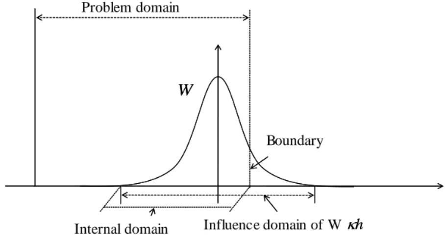
When the supporting domain is within the problem domain as shown in Fig. 2.1, the kernel function

10

W satisfies the compact condition, so the surface integral on the right side of equation (2.2.14) is zero.

However, on the other hand, in the case of Figure 2.2 where the supporting domain is partially outside the problem domain, the kernel function W is cut off by the boundary, and the surface integral is no longer zero. Under such circumstances, if the surface integral in equation (2.2.14) is zero, the boundary effect needs to be improved. Assuming that the points in the supporting domain are all in the problem domain, equation (2.2.14) can be simplified as follows.

















 f(x) f(x') W(x x',h)dx' (2.2.15) From the above equation, in the integral representation of the derivative of the SPH field function, the spatial gradient is determined from the value of the function and the derivative of the kernel function rather than the derivative of the function itself.

h W

Ｗの影響領域 問題領域

境界

内部領域 h

W

Ｗの影響領域 問題領域

境界

内部領域 Problem domain

Internal domain Influence domain of W Boundary

Fig 2.1 The kernel function supporting domain in the problem domain W

h Ｗの影響領域

問題領域

W

h Ｗの影響領域

問題領域

Influence domain of W Problem domain

Fig 2.2 The supporting domain of the kernel function intersects with the problem domain

11

2.2.3 Particle approximation

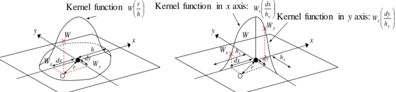
In the SPH method, the entire system is represented by a finite number of particles with individual mass and volume (area), which is a very important operation in the SPH method. In SPH kernel approximation, the continuous integral representation expressed by equations (2.2.4) and (2.2.15) can be approximated to the sum of all particles in the affected area as shown in Fig. 2.3. In the figure, W:

kernel function, Ω: influence region, 𝜅ℎ : influence radius, 𝑟_𝑖𝑗: inter-particle distance.

The discretization process corresponding to the sum of particles is generally known as particle approximation in SPH papers, and this process is described below.

First, replace the infinitesimal value dx' of the particle j integral with the particle finite volume Vj

 related to the particle mass m_j. Here, m_j is expressed by the following equation.

j j

j V

m   (2.2.16)

In the above equation, _j is the density of particles j (= 1, 2, ...,). N is the number of particles in the affected area of particle j. A continuous SPH integral representation for f(x) and can be written in the form of a discretized particle approximation such as

Fig 2.3 The influence domain circle of particle i



 h W

i j r

ij



 h W

i

j

r

ij

12

) 1 ( ) , ( ) (

) 1 (

) , ( ) (

) , ( ) (

' ) , ' ( ) ' ( )

(

1 1 1

j j j N

j j

j j j j N

j j

j j

N

j j

m h

x x W x f

V h

x x W x f

V h x x W x f

dx h x x W x f x f



 





































　　 　　 　　

(2.2.17)

Or，

) , ( ) ( )

(

1

h x x W x m f x

f _{j j}

N

j j

j 









^(2.2.18)

The particle approximation is derived as shown above. Thus, the particle approximation of the function at particle i can be finally expressed as

_{j ij}

N

j j

j

i m f x W

x

f 







) ( )

(

1



^(2.2.19)

where

) , (x x h W

W_ij  _i  _j (2.2.20)

Equation (2.2.19) indicates that the value of the function at particle i is approximated using the average of all particle values within the smoothing length of particle i weighted by the kernel function.

Similarly, the particle approximation in the spatial differentiation of the function can be expressed as ( ) ( ) ( , )

1

h x x W x

m f x

f _{j j}

N

j j

j  











  ^(2.2.21)

Here, the gradient W in the above equation depends on the particle j. Therefore, the particle approximation of the function at particle i can be finally expressed as

_{j i ij}

N

j j

j

i m f x W

x

f  









) ( )

(

1  ^(2.2.22)

where

ij ij ij ij ij

ij ij

j i ij

i r

W r x r W r

x W x



 





 

 (2.2.23)

Equation (2.2.22) shows that the gradient value of the function at particle i is approximated using the average of all particle values in the region of influence of particle i weighted by the gradient of the kernel function.

Particle approximation can be conveniently applied to hydrodynamic problems where density is an

13

important field variable by introducing particle mass and density into the equation. This is one of the main reasons why the SPH method is particularly used in dynamic flow problems. If the SPH particle approximation can be applied to solid mechanics problems, special handling is considered necessary.

In addition, particle approximation is related to numerical problems specific to SPH method such as particle inconsistency and stretchable instability. It is said that the number of reference points for integration should be larger than the field nodes (particles) to eliminate these problems.

For particle approximation, given particle i, the function value and its derivative are approximated at particle i as follows.

_{j ij}

N

j j

j

i m f x W

x

f( ) ( )

1





  ^(2.2.24)

_{j i ij}

N

j j

j

i m f x W

x

f  









) ( )

(

1  ^(2.2.25)

W_ij W(x_i x_j,h)W(x_i x_j,h) (2.2.26)

ij ij ij

ij ij

ij ij

j i ij

i r

W r x r W r

x W x



 





 

 (2.2.27)

where r_ij is the distance between particle i and particle j. Since _iW_ij is determined by the particle i, the negative sign in Eq. (2.21) is removed in Eq. (2.2.25). If we replace function f(x) with density

 in equation (2.2.24), the SPH approximation for density is

_ij

N

j j

i



m W





1



(2.2.28)

Equation (2.2.28) is the most general formula for obtaining the density with SPH, which is the sum density, and indicates that the particle density is the average of the weighted densities of all particles in the affected area.

2.2.4 Formulation method of SPH

By using the kernel approximation and particle approximation procedures described above, the formulation of SPH by partial differential equations can always be derived. There are many methods for deriving SPH formulation using partial differential equations, but a simpler method is used directly

14

using equations (2.2.24) and (2.2.25). This method uses the following two expressions to define the density within the gradient operator.

  ^  ^ 



^{  }





 1 ( ) ( )

)

(x f x f x

f (2.2.29)



 



  











 

( )) ⁽₂⁾ (

)

( f x f x

x

f (2.2.30)

The above two equations are substituted into the integral of equation (2.2.11), and the gradient term on the right side of equations (2.2.29) and (2.2.30) is applied as the same procedure as particle approximation of equation (2.2.25). Each equation outside the gradient term uses the particle's own value, and the following equation is obtained from the result of f(x) divergence for particle i obtained from equations (2.2.29) and (2.2.30).

 

_



 



  









 N

j

ij i i j

j i

i m f x f x W

x f

1

) ( ) 1 (

)

(  ^(2.2.31)











 















 















 







 N

j

ij i i

i j

j j

i

i f x f x W

m x

f

1

2 2

) ) (

) (

(    (2.2.32)

One of the advantages of the above two formulas is that the field function appears in the form of a pair of particles.

In addition to the two equations described above, there are other useful operational rules that can be used to derive SPH equations for complex systems. For any two functions of field variables f₁ and

f2, the following rules exist:

f₁ f₂  f₁  f₂ (2.2.33)

f₁f₂  f₁ f₂ (2.2.34)

Therefore, the SPH approximation of the sum of the functions and the sum of the SPH approximation of each function is equal, and the SPH approximation of the functions multiplied and the product of the SPH approximation of each function is equal.

2

2 c f

cf  (2.2.35)

Equations (2.2.33) and (2.2.35) mean that the SPH approximation operator is a linear operator. It is

15

easy to understand that the SPH approximation operator is commutative, and can be expressed as

f₁ f₂  f₂ f₁ (2.2.36)

f₁f₂  f₂f₁ (2.2.37)

2.3 Kernel function

2.3.1 Conditions of kernel function

Section 2.2 described the basic concept and important formulation of the SPH method. In the SPH approximation, the kernel function plays an important role in determining the accuracy and efficiency of the computation.

Here, a general method for constructing the kernel function in the SPH method is shown. In the method, a well-formed expression using Taylor series expansion is used. A set of conditions is systematically derived and used to construct both kernel functions and point-dependent kernel functions in the analysis given in numerical form. These conditions not only ensure consistency in the SPH approximation, but also represent the compact support condition for the kernel function.

One of the main problems of the mesh-free method is to perform function approximation based on nodes that are scattered efficiently and arbitrarily without pre-defining meshes and grids that provide node connectivity. Methods for approximating functions fall into three categories. The three are 1) integral representation, 2) series representation, and 3) difference representation. The SPH method uses integral representation with the kernel function. The kernel function is a very important factor because it determines the type of function approximation and not only defines the range of the particle influence area, but also the consistency and accuracy of the kernel approximation and particle approximation.

In SPH method, different kernel functions are used, while these kernel functions satisfy the same conditions and are with same characteristics although the function types are different. The main characteristics are described below.

1. The kernel function must be standardized (Unity condition)



W(xx^',h)dx^' 1 (2.3.1)

16

2. kernel functions should be represented in a certain region (Compact support), h

x x for x

x

W(  ^')0,  ^'  (2.3.2)

The compact support domain is defined by the kernel function h and the coefficient kappa.

Where h is the smoothing length and kappa determines the spread of a specific kernel function.

3. W(xx')0 holds for any point 'x in the region of influence of the particle at any point x (positive value).

4. The value of the kernel function for a particle generally decreases monotonically as the distance from the particle increases. (Attenuation)

5. The kernel function satisfies the Dirac delta function condition when the smoothing length approaches 0 (the characteristics of the delta function).

) ' ( ) , ' (

lim0W x x h x x

h   





(2.3.3)

6. The kernel function is an even function (Symmetric) ． 7. The kernel function is smooth enough (Smoothness)

The first “Unity condition” means that the integral value of the kernel function in the support domain is 1.

The second condition is responsible for converting the SPH approximation from global to local.

Because this condition leads to an arbitrarily distributed calculation matrix, this condition is largely related to the computing power of the computer.

The third condition means that the kernel function value should not be negative in the support area.

This is not necessary for mathematically converging calculations, but for stabilizing physical phenomena.

The fourth condition is based on the physical idea that particles that are close to the particle being considered should have a significant influence to each other. That is, as the distance between two interacting particles increases, the force acting between the two interacting particles decreases.

However, this condition is not satisfied for an object in which the influence force increases as the distance between two particles increases.

As for the fifth condition, it can be satisfied as the smoothing length approaches zero. This condition is naturally satisfied by satisfying conditions 1 to 4.

17

The sixth condition means that particles that are located at different locations for a particle but have the same distance have the same effect on a particle. This is not an absolutely necessary condition and may not be met by the highly invariant mesh-free particle method.

The seventh condition is for obtaining an accurate approximation. To obtain accurate results in function and derivative approximations, the kernel function should always be continuous. A kernel function with a smooth function and derivative value generally yields good results. This is because the kernel function does not affect irregularly arranged particles and the approximation error of the integral interpolation formula is reduced.

A function with the above characteristics is used as the kernel function of the SPH method. Many researchers devise and use different types of kernel functions. Some of the kernel functions used in SPH literature are listed in the following section.

2.3.2 Typical example

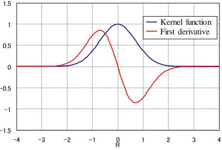
Monaghan⁴⁾ states that it is best to use a Gaussian distribution for the kernel function to obtain a physical interpretation in the SPH formulation. Gingold and Monaghan⁵⁾ adopted the following Gaussian kernel shown in Fig. 2.4.

) 2

,

(R h _de ^R

W  ^ (2.3.4)

where _d=1/^1/2h,1/h²,1/^3/2h³, in 1D, 2D, 3D space, respectively.

The Gaussian kernel is considered the best kernel function because even higher-order derivatives are sufficiently smooth, and the calculations are accurate and stable for irregularly moving particles.

However, even if R approaches infinity, W is not theoretically zero, so it cannot be said to be truly compact. In addition, it must be noted that this function is the most computationally expensive because calculation domain is too large. In particular, this applies to all higher-order derivatives of the kernel function, which requires a broad support domain containing many particles in the particle approximation and requires the ability to process individual computational matrices.

18

Fig 2.4 Gaussian kernel and first derivative

Based on a cubic spline function, Monaghan and Lattanzio⁶⁾ devised a kernel function called “B- spline function” shown below.

   







































R R R

R R

R

h R

W _d

2 0

2 1

6 2 1

1 2 0

1 3

2

, ³

3 2



(2.3.5)

where



_d

 1 / h

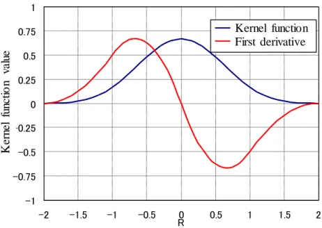
,15/7h², 3/2h³ , in 1D, 2D, 3D space, respectively.

The cubic spline function is similar to the Gaussian kernel and is the most widely used kernel function so far because it can provide a narrower compact support than the Gaussian kernel. However, since the second derivative of the cubic spline function is piecewise linear, the stability characteristics are inferior to other functions. In addition, the kernel function is defined for three ranges, which is slightly more difficult than a kernel function consisting of one function.

-1.5 -1 -0.5 0 0.5 1 1.5

-4 -3 -2 -1 0 1 2 3 4

R

関数値

kernel関数 導関数

Figure 2.4 Gaussian kernel and first derivative -1.5

-1 -0.5 0 0.5 1 1.5

-4 -3 -2 -1 0 1 2 3 4

R

関数値

kernel関数 導関数

Kernel function First derivative

19

Fig 2.5 Cubic spline function and first derivative

Morris^7,8) proposed a higher-order spline function that is closer to the Gaussian kernel and more stable.

Here, the quintic spline function is shown in equation (2.3.6).

































0 ) 3 (

) 2 ( 6 ) 3 (

) 1 ( 15 ) 2 ( 6 ) 3 ( )

,

( ₅

5 5

5 5

5

R

R R

R R

R h

R

W _d

3 3 2

2 1

1 0















R R R

R

(2.3.6)

where _d=120/h, 7/478h², 3/359h³, in 1D, 2D, 3D space, respectively.

2.4 Numerical aspects

In the SPH method, artificial viscosity is added to stabilize the calculation. The details are explained here. Influence radius directly related to analysis accuracy is also introduced.

2.4.1 Artificial viscosity

To simulate fluid mechanics problems, special measures and methods are needed to allow the modeling of shock waves that amplify non-physical vibrations in numerical results. Although the shock wave is not discontinuous in reality, it is a parallel free path in a very limited displacement region with a thickness of a few molecules. Application of mass, momentum, and energy conservation conditions to the front of the shock wave requires a simulation of conversion of kinetic energy to thermal energy,

-1 -0.75 -0.5 -0.25 0 0.25 0.5 0.75 1

-2 -1.5 -1 -0.5 0 0.5 1 1.5 2

R

関数値

kernel関数 導関数

-1.5 -1 -0.5 0 0.5 1 1.5

-4 -3 -2 -1 0 1 2 3 4

R

関数値

kernel関数 導関数

Kernel function First derivative

Kernel function value

20

and physically this energy conversion is expressed as viscous dissipation. This idea leading to the development of von Neumann-Richtmyer artificial viscosity is expressed by equation (2.4.1).

 





















 



0 0

2 0

2 1

1 v

v v

x

a



(2.4.1)

where ₁ is von Neumann-Richtmyer artificial viscosity and is required during material compression.

a1 is an adjustable dimensionless constant. von Neumann-Richtmyer artificial viscosity is the second- order term of velocity derivative.

It was also discovered that the addition of the linear artificial viscosity term ₂ expressed by Eq.

(2.4.2) has the advantage of smoothing vibrations that cannot be suppressed by secondary artificial viscosity.





















 

 0 0

2 0

2 v

v v

xc

a



(2.4.2) where c is the speed of sound and is a₂ an arbitrary constant.

The second-order von Neumann-Richtmyer artificial viscosity ₁ and linear artificial viscosity

2 are widely used in fluid dynamics analysis to eliminate numerical vibrations. The artificial viscosity term serves to normalize numerical instabilities caused by (discontinuous) sharp fluctuations by spreading the shock wave into several meshes. Also, the artificial viscosity term is often added to the physical pressure term to diverge sudden fluctuations at transitions and help diffuse energy at high vibration terms.

The SPH method was first applied to deal with low-loss or no-loss problems, and then developed to simulate impact problems by Monaghan and Gingold⁹⁾. This Monaghan type artificial viscosity _ijis the most widely used artificial viscosity in SPH papers. This not only defines the loss required to convert kinetic energy into thermal energy in front of the shock wave, but also prevents non-physical, close-up penetration of each other's particles. The detailed formula is described below.













 











0 0

0

2

ij ij

ij ij ij

ij ij

ij ij

x v

x c v











(2.4.3)

where

21

2 2

 



 

ij ij ij ij ij

x x v

h (2.4.4)



_{i j}



ij c c

c  

2

1 (2.4.5)



i j



ij

 



 

2

1 (2.4.6)



_{i j}



ij h h

h  

2

1 (2.4.7)

j i ij j i

ij v v x x x

v   ,   (2.4.8)

where _, _ are coefficients and are often 1.0

The coefficient 0.1h_ij is included to prevent numerical divergence when two particles approach each other. c and v represent the sound velocity and particle velocity vectors, respectively. Viscosity related to _ gives rise to volume viscosity, while the second term related to _ to suppress interpenetration of particles at high Mach numbers is similar to the von Neumann-Richtmyer artificial viscosity.

In addition, Monaghan-type artificial viscosity introduced shear viscosity into the flow, especially in the region away from the impact field, and the artificial viscosity based on the velocity field derivative was used by Hernquist and Katz¹⁰⁾.

2 2

j j i

i ij

q q



 ^



 (2.4.9)

where



























 ^  ^

0 0

2 0

2

i i i

i i i

i i i

i v

v v

h v

c

q  h  

(2.4.10)

2.4.2 Smoothing length

The smoothing length is very important in SPH method because it directly affects the efficiency of the calculation and the accuracy of the solution. If it is too small, there will be insufficient particles within the supporting domain, and the result will be less accurate. On the other hand, if it is too large, the micro-changes and local properties of the particles will probably be smoothed and inaccurate. The particle approximation used in the SPH method depends on the number of sufficient and necessary

22

particles present in the supporting domain. The time and speed of the calculation also depend on the number of particles. In 1, 2 and 3 dimensions, if the particles are located in a grid and the radius of influence is 1.2 times the distance between the particles, then the number of surrounding particles is about 5, 21, and 57, respectively.

In the early stage of SPH, the overall particle radius was used depending on the initial average density of the system. Later, the influence radius can be solved by assigning individual influence radius determined by small changes in density in each particle, thereby maintaining consistent accuracy throughout the space and solving the problem of local expansion or contraction of the liquid. For anisotropic problems such as impact problems, the radius of influence is required to change with both space and time.

There are many ways to dynamically expand h so that the number of surrounding particles is relatively constant. The simplest method is to update the radius of influence using the average density

d

h h

1 0 0 

 



 



 (2.4.11)

where h₀ and ₀ are the initial smoothing length and density, respectively. d is the number of dimensions.

Benz¹¹⁾ proposed another method of expanding the smoothing length by incorporating the time derivative of the kernel function into a continuous equation.

dt d h d dt

dh





1

 (2.4.12)

Equation (2.4.12) is discretized using the SPH approximation and computed in parallel with other differential equations

2.4.3 Symmetry of interaction

If the smoothing length varies with both space and time, each particle has its own smoothing length.

If h_i is not equal to h_j, the region of influence of particle i may extend to particle j, but not vice versa. In addition, particle i can exert a force on particle j even if particle j does not have a corresponding action on particle i. But this relationship violates Newton's third law. In order to solve this problem, several measures were required to maintain the symmetry of the particle interaction. Here, a method to improve the smoothing length is described. There are different ways to improve the symmetry radius

23

in order to maintain interaction contrast. One way to calculate a symmetric smoothing length is to take the arithmetic mean or average of a pair of smoothing length of interacting particles.

2

j i ij

h h h 

 (2.4.13）

In addition, a method of calculating the smoothing length using the geometric mean of the smoothing length of a pair of interacting particles is also used.

j i

j i

ij h h

h h h

 2

(2.4.14) Or take the maximum of h_i and h_j as the smoothing length



i j



ij h h

h max , (2.4.15)

Or take the minimum of h_i and h_j as the smoothing length



i j



ij h h

h min , (2.4.16)

Furthermore, the kernel function is obtained from using the symmetric smoothing length



ij ij



ij W r h

W  , (2.4.17)

There are advantages and disadvantages to these different ways of determining the symmetric smoothing length h_ij. When using the arithmetic mean of equation (2.4.13) or the maximum smoothing length of equation (2.5.15), there is a tendency to use more surrounding particles and to overly smooth the effects between surrounding particles. In addition, when using the geometric mean of equation (2.5.14) or the minimum value of the smoothing length of equation (2.4.16), it is necessary to be careful because fewer surrounding particles are used. In addition, as an alternative method of maintaining particle interaction, the average of kernel function values is used directly without using the symmetric smoothing length.

   



i j



ij W h W h

W  

2

1 (2.4.18)

These equations are widely used in SPH that preserves particle interactions.

24

25

Chapter 3 Application of SPH in numerical analysis

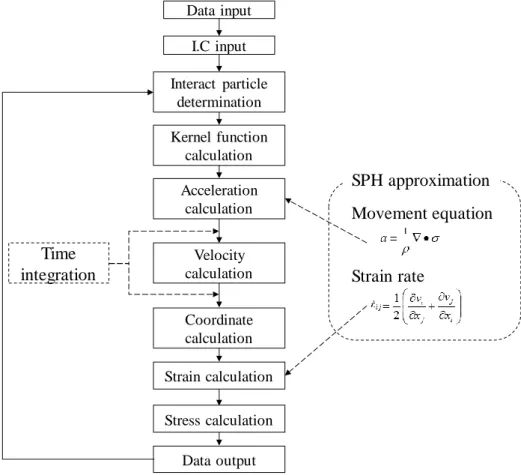
3.1 Analysis procedure of SPH method

In the SPH method in this study, calculations are conducted according to the flow shown in Fig. 3.1.

Fig 3.1 Analysis procedure

3.2 Particle approximation

3.2.1 Basic theory and formula of ASPH method

The general SPH method uses a uniform kernel function in all directions, but here we outline the ASPH method using a kernel function that expresses anisotropy. In this study, the crack model with stress release and anisotropic constitutive law is adopted. The crack model is implemented by the effect

Data input I.C input Interact particle

determination Kernel function

calculation Acceleration

calculation Velocity calculation Coordinate calculation Strain calculation Stress calculation

Data output Time

integration

SPH approximation Movement equation

Strain rate