九州大学学術情報リポジトリ
Kyushu University Institutional Repository
沿岸域環境における粒状態水銀動態の数値モデリン グ:水俣湾におけるケーススタディ
エディストリ, ヌル, ファティヤ
https://doi.org/10.15017/1866309
出版情報:Kyushu University, 2017, 博士(工学), 課程博士 バージョン:
権利関係:
NUMERICAL MODELING OF PARTICULATE MERCURY DYNAMICS IN COASTAL
ENVIRONMENT:
CASE STUDY IN MINAMATA BAY, JAPAN
Edistri Nur FATHYA
Numerical Modeling of Particulate Mercury Dynamics in Coastal Environment:
Case Study in Minamata Bay, Japan
A Doctoral Thesis Submitted In Partial Fulfilment of the Requirements
For the Degree of Doctor of Engineering
By
Edistri Nur FATHYA
to the
DEPARTMENT OF MARITIME ENGINEERING GRADUATE SCHOOL OF ENGINEERING
KYUSHU UNIVERSITY
2017
DEPARTMENT OF MARITIME ENGINEERING GRADUATE SCHOOL OF ENGINEERING
KYUSHU UNIVERSITY Fukuoka, Japan
CERTIFICATE
The undersigned hereby certify that they have read and recommend to the Graduate School of Engineering for the acceptance of this doctoral thesis entitle “Numerical Modeling of Particulate Mercury Dynamics in Coastal Environment: Case Study in Minamata Bay, Japan” by Edistri Nur FATHYA in partial fulfillment of the requirements for the degree of Doctor of Engineering.
Dated: July, 2017 Thesis Supervisor:
______________________________________
Prof. Shinichiro YANO, Dr. Eng.
Examining Committee:
______________________________________
Prof. Noriaki HASHIMOTO, Dr. Eng.
_______________________________________
Prof. Takahiro KUBA, Dr. Eng.
i
Abstract
Minamata disease was a one of huge tragedy that claimed many victims in Japan in 1956. The disease was caused by mercury contamination which disposed by a chemical factory to the Minamata Bay. The inorganic mercury that had been used for acetaldehyde formation, were disposed and this compound could transform into methylmercury (MeHg) compound. MeHg is the most toxic compound of mercury which accumulates in the marine organism and also human who consumed it. Around 40,000 people were reported affected by this disease, which attacked central nervous system. The MeHg compound itself is mostly found at sediment in the bottom layer.
Therefore to solve this problem, Japanese government had conducted remediation project to remove the contaminated bottom sediment around Minamata Bay. Bottom sediment which contained more than 25 ppm of mercury was removed and reclaimed to the enclosed area in the bay.
Many years after the project, the transport of particulate mercury from Minamata Bay to the outer side of the bay was reported. The transport was expected came from the remaining mercury in bottom sediments in Minamata Bay which was not been removed (less than 25ppm concentration). Mercury was found in the Yatsushiro Sea, the western sea from the bay, and also some Minamata disease victim were found in Amakusa region in the western part of the Yatsushiro Sea. Numerical simulations and field measurement of sediment transport from Minamata Bay also have shown that there is transport to the Yatsushiro Sea. Yano et al. (2014) had conducted the sediment transport simulation, and showed result of the western, southern, and northern transport due to the flow. However, the description of the bay from their simulation was not precise yet.
In order to get better and accurate result, this research suggests using a better resolution
ii
grid of the bay and other considered model parameters. In addition, it is also necessary to understand mercury fate in sediment, and also the mechanism of its transport in the coastal environment.
The present research is divided in some chapter in this thesis, and described as follow:
Chapter 1 explains about research background, research problem, research objectives, the scope of the research, and also the overview of the thesis as an introduction.
Chapter 2 explains about mercury dynamics in the global environment, including its cycle. Furthermore, mercury problem includes Minamata disease outbreak and also the solution are described. The three-dimensional numerical model of hydrodynamics and sediment transport by Delft3D is also presented.
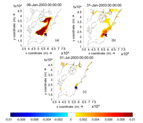
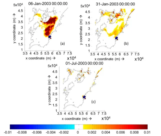
Chapter 3 presents numerical simulation using a new grid system and additional layers for simulating sediment transport in Minamata Bay. The rectangular variable grid is divided into three different grid sizes, namely, 250m (original size), 125m, and the finest 62.5m. The sediment transport and tidal flow are calculated. In this chapter, the previous simulation by Yano et al. (2014) is compared with the result of the new variable grid system. The results show that by adapting the additional layers and the finer grid, there is a northward movement of sediment around the coastal area. From six months simulation, it is showed that most deposit areas that generated by barotropic flow are the western and southern area from Minamata Bay and baroclinic flow moves the sediment to north and finally dispersed it to outside area of the southern Yatsushiro Sea.
Chapter 4 discusses the impact of the reclamation project in mercury highly-
contaminated sediment in Minamata Bay. Here also tidal flow and sediment transport
are simulated and applied in two different topography before and after reclamation
around the bay. The change of hydrodynamic condition inside of the bay due to the
remediation project gives a slight change in sediment transport pattern. It is estimated
that the sediment after the reclamation can transport slower than before it because of
change of its magnitude of velocity above the seabed. It is clarified that a change of the
amount of bottom sediment which can be re-suspended in the bay due to the
topographical change can also affect the pattern. Also, this result suggests that the
iii
southern part of Yatsushiro Sea can be influenced by sediment contaminated by higher Hg included before the reclamation project.
Chapter 5 simulates the effect of the damage of reclamation walls in Minamata Bay.
The walls that built more than 25 years ago, when the remediation project has been conducted, is feared to be collapsed and leaked highly contaminated mercury from the reclamation area to the bay. In order to predict an influence of sediment leakage, the numerical simulation of sediment transport and suspended solid (SS) distributions from the reclaimed wall area to the bay are conducted. We assume a part of the wall in the north and south part collapsed and for one day in rainy season, the highly contaminated sediments including mercury are released to the bay. SS distribution to the bay is more significant when the south part of reclamation wall collapses than the north part. In the upper layer, when the low tide occurs, barotropic and baroclinic flows move SS to southwest direction entering the bay, and at high tide, the SS can be distributed around the northern area. From the result, in the upper layer, it can be assumed that baroclinic flow is significantly distributing SS to Minamata Bay, meanwhile in the deeper layer barotropic and baroclinic flow almost have a similar contribution in transporting the sediment from reclamation wall to the bay.
Chapter 6 evaluates the relationship between particulate total mercury (P-THg) in seawater and suspended solids particle size distribution in Minamata Bay. We used a cluster analysis by the Ward method, attempted to judge the best grouping using the entropy method, and confirmed statistical significance of the relationship between each group and P-THg concentration with both of Bartlett test and Kruskal-Wallis test. The results show that the most optimal group number of SS particle size distribution was determined as six groups, also statistically significant correlation between the P-THg concentration and SS particle size distribution was seen and from the present relationship between particulate THg concentration and SS particle size fraction, that particulate THg depends on source of SS and mixing condition with SS from rivers and other possible sources.
Chapter 7 concludes all chapters in this thesis and also proposes some recommendation
for future works.
iv
Acknowledgement
“Then, surely with hardship comes ease,”
“Surely, with hardship comes ease.”
Qur’an (94: 5-6)
Alhamdulillah…
Praise to Allah SWT for all his mercy and compassion, so that I could finish my study by publishing this thesis.
Firstly, I owe my deepest gratitude for Prof. Shinichiro Yano as my supervisor for guiding and helping me during my study in Kyushu University. Thank you for believing me to do this research and thank you for the time, advice, encouragement, and also attention not only about academic things but also about my life during my stay in Japan.
Also, I would like to express my sincere gratitude for the committee member, Professor Noriaki Hashimoto and Prof. Takahiro Kuba for the time, suggestion and improving comment to finish this thesis. Thanks also to Associate Prof. Tai and Dr. Kimura for the help and recommendation during my study and research in Kyushu University and Dr. Oshikawa and Dr. Hashimoto for the help during my early years I stay in the laboratory.
I would like to express my gratitude to Dr. Akito Matsuyama from National Institute of Minamata Disease and Dr. Akihide Tada from Nagasaki University for the collaboration of research, also for teaching and showing me how to conduct field and laboratory experiment of mercury in Minamata Bay.
Next, I would like to thanks to Ms. Kumamoto and Mr. Fujita for the help which could
indirect also helping me through the research and academic life in Kyushu University.
v
Thanks to Mr. Oiwa from International Student Support Center for all the help and guidance to make my study easier and also I acknowledge Japanese government to provide my scholarship through MEXT.
I also thanks to laboratory members during this 3 years, also the foreign students (Youtou, Lisa, Camila, Nga) for the hospitality, help and guidance to do the research also to get to know Japanese life, and for sharing the great memory during my study in Japan. Thanks to Pak Nasser for the sharing and help during the laboratory and doctoral student life.
Thanks to my Indonesian friends, my roommate, Sito and Sophia, thanks to PPIF (Indonesia-Fukuoka Student Association) and Muslimah Fukuoka as my third family in Japan for all the sharing, help and support, I could meet many kinds of people and have a new experience to live in foreign country and I also thank everyone which whom I could not mention it here.
I would also express my gratitude for the company where I work in Indonesia, ASR, Ltd., Mr. Gegar, Ph.D. as the director, Dr. Rahman and Dr. Fitri as the alumnus from Kyushu University and other colleagues, thanks for the opportunity, support, and convincing me to continue my study in Japan. I also thank all the lecturers and my supervisor from Department of Oceanography and Earth Sciences in Bandung Institute of Technology for all support, guidance, and for introducing me to oceanography and earth sciences during undergraduate and master.
Finally, thanks to my family, my father for the big support, my mother for her sacrifice and big help for me especially in the last semester of my study, my sister, my husband, and also my little baby who could give me strength and realize me that being a mother and also third-year doctoral student is beyond my expectation but we could get through all of it.
Edistri Nur Fathya
Fukuoka, July 2017
vi
Contents
Abstract ... i
Acknowledgement ... iv
Contents ... vi
List of figures ... ix
Chapter 1 Introductions ... 1
1.1 Research Background ... 1
1.2 Research problem ... 4
1.3 Research Objectives ... 5
1.4 Scope of the study ... 6
1.5 Overview of the thesis ... 7
References ... 9
Chapter 2 Mercury Dynamics in Natural Environment ... 11
2.1 Mercury in global environment ... 11
2.1.1Source of mercury emission to air and water ... 12
2.1.2 Global mercury budget ... 13
2.2 Mercury cycle ... 16
2.3 Mercury problems ... 20
2.3.1 Mercury contamination in the world ... 20
2.3.2 Mercury contamination in Minamata Bay ... 21
2.3.2.1 Minamata disease outbreak ... 21
2.3.2.2 Geographical and oceanographic condition in Minamata Bay and the Yatsushiro Sea ... 23
2.3.2.3 Remediation project of Minamata Bay ... 24
2.4 Modeling of Mercury Transport in Bottom Sediment ... 27
2.4.1 Numerical model description ... 27
vii
2.4.2 Hydrodynamic model equation ... 28
2.4.3 Transport model equation ... 28
2.4.4 Erosion and deposition equation ... 30
References ... 31
Chapter 3 Numerical Simulation of Fine Sediment Transport in Minamata Bay Using Variable Grid ... 35
3.1 Introduction ... 36
3.2 Model Description ... 38
3.2.1 Computational domain ... 38
3.2.2 Variable grid system ... 38
3.2.3 Numerical model description ... 40
3.2.4 Input Parameter ... 40
3.3 Result and Discussion ... 42
3.3.1 Result in 5 layers case ... 42
3.3.2 Result in 10 layers case ... 44
3.3.3 Comparison between 5 layers and 10 layers result ... 46
3.4 Conclusions ... 49
References ... 50
Chapter 4 Impact of Reclamation Project on Mercury-Contaminated Sediment Transport from Minamata Bay into the Yatsushiro Sea ... 52
4.1 Introduction ... 53
4.2 Model Description ... 55
4.2.1 Computational domain and grid system ... 55
4.2.2 Numerical Model ... 56
4.2.3 Boundary conditions and model parameters ... 56
4.3 Validation of Simulations ... 58
4.3.1 Validation of water level ... 58
4.3.2 Validation of horizontal distribution of cumulative sediment ... 59
4.4 Result and Discussion ... 60
4.4.1 Hydrodynamic conditions in before and after reclamation cases ... 60
4.4.2 Bottom sediment transport in before and after reclamation cases ... 62
4.5 Conclusions ... 65
References ... 66
viii
Chapter 5 Evaluation of the Effects of the Damage of Reclamation Wall on Sediment Transport and Suspended Solid
Distribution in Minamata Bay ... 68
5.1 Introduction ... 69
5.2 Numerical Modeling ... 71
3.2.1 Computational domain and grid ... 71
5.2.2 Calculation method ... 72
5.2.3 Boundary conditions, input parameter and scenarios ... 73
5.3 Result and Discussions ... 75
5.3.1 Result of suspended solid distribution ... 75
5.3.1.1 South wall damage ... 75
5.3.1.2 North wall damage ... 77
5.3.1.3 Suspended solid transport after 30 days ... 79
5.3.2 Result of sediment transport ... 81
5.4 Conclusions ... 84
References ... 86
Chapter 6 Evaluation on Relationship between Particulate Total Mercury in Seawater and Suspended Solids Particle Size Distribution in Minamata Bay, Japan ... 88
6.1 Introduction ... 89
6.2 In-Situ Measurement for Mercury Concentration and SS Grain Size Distribution in Seawater ... 91
6.3 Analysis of Measurement Data ... 93
6.3.1 Grouping of SS grain size distribution data ... 93
6.3.2 Evaluation of Statistical Significance ... 96
6.3.3 Evaluation of Relationship between Specific Surface Area of SS and Particular THg Concentration ... 97
6.4 Conclusions ... 100
References ... 101
Chapter 7 Conclusion and Recommendation ... 103
ix
List of Figures
Figure 2.1. Global Mercury Budget [Unit: Mg/year] ... 14
Figure 2.2. Biogeochemical cycle of Mercury ... 16
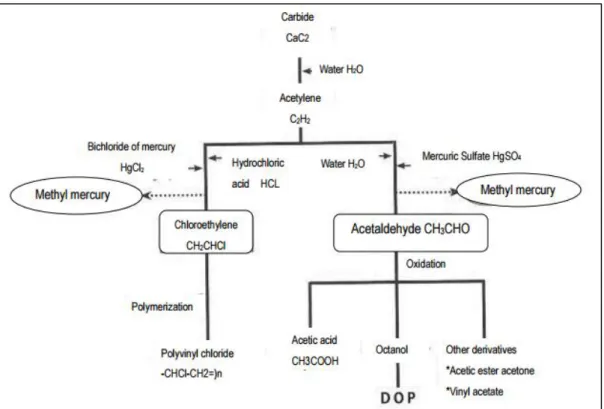
Figure 2.3. Methylmercury formation in Chisso Factory, Minamata ... 21
Figure 2.4. Mercury biomagnification and bioaccumulation mechanism in Minamata ... 22
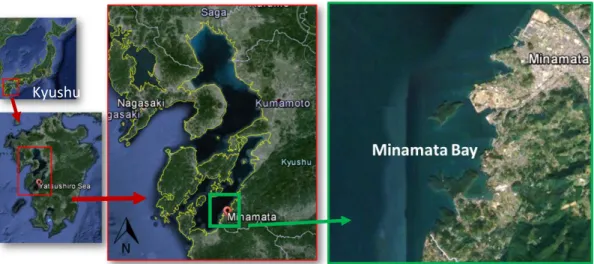
Figure 2.5. Map of Ariake and Yatsushiro Sea, Japan ... 24
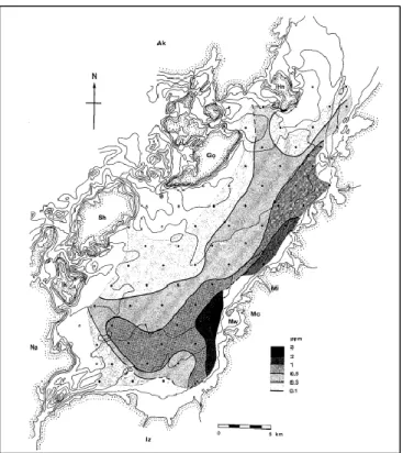
Figure 2.6. Distribution of the maximum mercury content (ppm)... 26
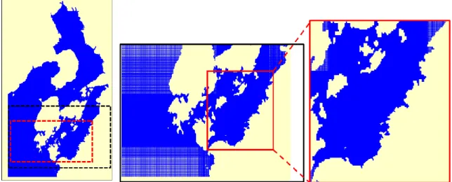
Figure 3.1. Computational domain and area of the Yatsushiro Sea ... 38
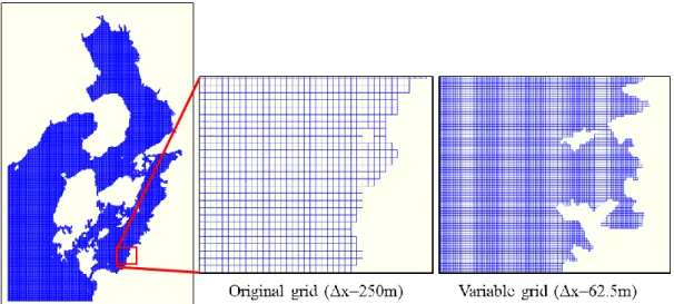
Figure 3.2. Variable grid system in the computational domain ... 39
Figure 3.3. Comparison of grid size in Minamata Bay, left: original grid (250m), right: variable grid (62.5 m) ... 40
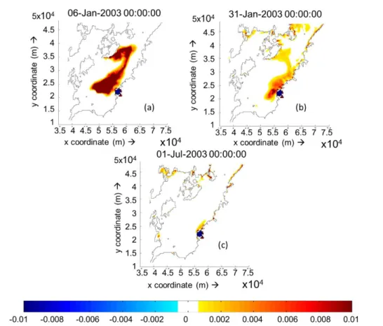
Figure 3.4(a). Cumulative deposition and erosion thickness on 5 layers simulation without freshwater inflow after 5days. [Unit: m] ... 43
Figure 3.4(b). Cumulative deposition and erosion thickness on 5 layers simulation without freshwater inflow after 30 days. [Unit: m] ... 43
Figure 3.4(c). Cumulative deposition and erosion thickness on 5 layers simulation without freshwater inflow after 180days. [Unit: m] ... 43
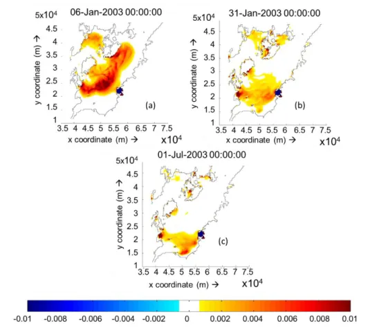
Figure 3.5(a). Cumulative deposition and erosion thickness on 5 layers simulation with freshwater inflow after 5days. [Unit: m] ... 44
Figure 3.5(b). Cumulative deposition and erosion thickness on 5 layers simulation with freshwater inflow after 30days. [Unit: m] ... 44
Figure 3.5(c). Cumulative deposition and erosion thickness on 5 layers simulation
without freshwater inflow after 180days. [Unit: m] ... 44
x
Figure 3.6(a). Cumulative deposition and erosion thickness on 10 layers simulation without freshwater inflow after 5days. [Unit: m] ... 45 Figure 3.6(b). Cumulative deposition and erosion thickness on 10 layers simulation
without freshwater inflow after 30days. [Unit: m] ... 45 Figure 3.6(c). Cumulative deposition and erosion thickness on 10 layers simulation
without freshwater inflow after 180days. [Unit: m] ... 45 Figure 3.7(a). Cumulative deposition and erosion thickness on 10 layers simulation
with freshwater inflow after 5days. [Unit: m] ... 46 Figure 3.7(b). Cumulative deposition and erosion thickness on 10 layers simulation
with freshwater inflow after 30days. [Unit: m] ... 46 Figure 3.7(c). Cumulative deposition and erosion thickness on 10 layers simulation
without freshwater inflow after 180days. [Unit: m] ... 46 Figure 3.8(a). Vertical profile of northward residual currents in case 5 layers without
freshwater inflow. (Positive is northward) ... 48 Figure 3.8(b). Vertical profile of northward residual currents in case 5 layers with
freshwater inflow. (Positive is northward) ... 48 Figure 3.8(c). Vertical profile of northward residual currents in case 10 layers without freshwater inflow. (Positive is northward) ... 48 Figure 3.8(d). Vertical profile of northward residual currents in case 10 layers with
freshwater inflow. (Positive is northward) ... 48 Figure 3.8(d). Vertical profile of northward residual currents in case 10 layers with
freshwater inflow. (Positive is northward) ... 48 Figure 4.1. Variable grid system and topography around Minamata Bay before and
after reclamation ... 55
Figure 4.2(a). Water level validation at Midori River point. [Unit: m] ... 58
Figure 4.2(b). Water level validation at Kuma River point. [Unit: m] ... 58
Figure 4.3(a). Horizontal velocity above seabed at low tide before the reclamation
project. [Unit: m/s] ... 60
Figure 4.3(b). Horizontal velocity above seabed at flood tide before the reclamation
project. [Unit: m/s] ... 60
Figure 4.3(c). Horizontal velocity above seabed at high tide before the reclamation
project. [Unit: m/s] ... 60
xi
Figure 4.3(d). Horizontal velocity above seabed at ebb tide before the reclamation project. [Unit: m/s] ... 60 Figure 4.4(a). Horizontal velocity above seabed at low tide after the reclamation project. [Unit: m/s] ... 61 Figure 4.4(b). Horizontal velocity above seabed at flood tide after the reclamation project. [Unit: m/s] ... 61 Figure 4.4(c). Horizontal velocity above seabed at high tide and after the reclamation project. [Unit: m/s] ... 61 Figure 4.4(d). Horizontal velocity above seabed at ebb tide after the reclamation project. [Unit: m/s] ... 61 Figure 4.5(a). Cumulative deposition and erosion thickness distribution before the reclamation project after 5 days. [Unit: m] ... 62 Figure 4.5(b). Cumulative deposition and erosion thickness distribution before the reclamation project after 30 days. [Unit: m] ... 62 Figure 4.5(c). Cumulative deposition and erosion thickness distribution before the reclamation project after 180 days. [Unit: m] ... 62 Figure 4.6(a). Cumulative deposition and erosion thickness distribution after the reclamation project after 5 days. [Unit: m] ... 63 Figure 4.6(b). Cumulative deposition and erosion thickness distribution after the reclamation project after 30 days. [Unit: m] ... 63 Figure 4.6(c). Cumulative deposition and erosion thickness distribution after the reclamation project after 180 days. [Unit: m] ... 63 Figure 5.1. Computational domain, grid system, and Minamata Bay grid ... 72 Figure 5.2(a). SS distribution by the damage of south reclamation wall without freshwater inflow in surface layer at low tide on the neap tide ... 75 Figure 5.2(b). SS distribution by the damage of south reclamation wall without
freshwater inflow in surface layer at low tide on
the neap to spring tide ... 75
xii
Figure 5.2(c). SS distribution by the damage of south reclamation wall without freshwater inflow in surface layer at low tide on the spring tide ... 75 Figure 5.2(d). SS distribution by the damage of south reclamation wall without
freshwater inflow in surface layer at low tide on
the spring to neap tide ... 75 Figure 5.3(a). SS distribution by the damage of south reclamation wall without freshwater inflow in surface layer at high tide on the neap tide... 76 Figure 5.3(b). SS distribution by the damage of south reclamation wall without
freshwater inflow in surface layer at high tide on
the neap to spring tide ... 76 Figure 5.3(c). SS distribution by the damage of south reclamation wall without freshwater inflow in surface layer at high tide on the spring tide ... 76 Figure 5.3(d). SS distribution by the damage of south reclamation wall without
freshwater inflow in surface layer at high tide on
the spring to neap tide ... 76 Figure 5.4(a). SS distribution by the damage of south reclamation wall with freshwater inflow in surface layer at low tide on the neap tide ... 77 Figure 5.4(b). SS distribution by the damage of south reclamation wall with freshwater
inflow in surface layer at low tide on
the neap to spring tide ... 77 Figure 5.4(c). SS distribution by the damage of south reclamation wall with freshwater inflow in surface layer at low tide on the spring tide ... 77 Figure 5.4(d). SS distribution by the damage of south reclamation wall with freshwater
inflow in surface layer at low tide on
the spring to neap tide ... 77 Figure 5.5(a). SS distribution by the damage of south reclamation wall with freshwater inflow in surface layer at high tide on the neap tide ... 77 Figure 5.5(b). SS distribution by the damage of south reclamation wall with freshwater
inflow in surface layer at high tide on
the neap to spring tide ... 77
xiii
Figure 5.5(c). SS distribution by the damage of south reclamation wall with freshwater inflow in surface layer at high tide on the spring tide ... 77 Figure 5.5(d). SS distribution by the damage of south reclamation wall with freshwater
inflow in surface layer at high tide on
the spring to neap tide ... 77 Figure 5.6(a). SS distribution by the damage of north reclamation wall without freshwater inflow in surface layer at low tide on the neap tide ... 78 Figure 5.6(b). SS distribution by the damage of north reclamation wall without
freshwater inflow in surface layer at low tide on
the neap to spring tide ... 78 Figure 5.6(c). SS distribution by the damage of north reclamation wall without freshwater inflow in surface layer at low tide on the spring tide ... 78 Figure 5.6(d). SS distribution by the damage of north reclamation wall without
freshwater inflow in surface layer at low tide on
the spring to neap tide ... 78 Figure 5.7(a). SS distribution by the damage of north reclamation wall without freshwater inflow in surface layer at high tide on the neap tide... 78 Figure 5.7(b). SS distribution by the damage of north reclamation wall without
freshwater inflow in surface layer at high tide on
the neap to spring tide ... 78 Figure 5.7(c). SS distribution by the damage of north reclamation wall without freshwater inflow in surface layer at high tide on the spring tide ... 78 Figure 5.7(d). SS distribution by the damage of north reclamation wall without
freshwater inflow in surface layer at high tide on
the spring to neap tide ... 78 Figure 5.8(a). SS distribution by the damage of north reclamation wall with freshwater inflow in surface layer at low tide on the neap tide ... 79 Figure 5.8(b). SS distribution by the damage of north reclamation wall with freshwater
inflow in surface layer at low tide on
the neap to spring tide ... 79
xiv
Figure 5.8(c). SS distribution by the damage of north reclamation wall with freshwater inflow in surface layer at low tide on the spring tide ... 79 Figure 5.8(d). SS distribution by the damage of north reclamation wall with freshwater
inflow in surface layer at low tide on
the spring to neap tide ... 79 Figure 5.9(a). SS distribution by the damage of north reclamation wall with freshwater inflow in surface layer at high tide on the neap tide ... 79 Figure 5.9(b). SS distribution by the damage of north reclamation wall with freshwater
inflow in surface layer at high tide on
the neap to spring tide ... 79 Figure 5.9(c). SS distribution by the damage of north reclamation wall with freshwater inflow in surface layer at high tide on the spring tide ... 79 Figure 5.9(d). SS distribution by the damage of north reclamation wall with freshwater
inflow in surface layer at high tide on
the spring to neap tide ... 79
Figure 5.10(a). SS distribution after 30 days without freshwater inflow by the damage
of south reclamation wall in surface layer... 80
Figure 5.10(b). SS distribution after 30 days without freshwater inflow by the damage
of south reclamation wall in bottom layer. ... 80
Figure 5.10(c). SS distribution after 30 days without freshwater inflow by the damage
of north reclamation wall in surface layer. ... 80
Figure 5.10(d). SS distribution after 30 days without freshwater inflow by the damage
of north reclamation wall bottom layer ... 80
Figure 5.11(a). SS distribution after 30 days with freshwater inflow by the damage of
south reclamation wall in surface layer. ... 81
Figure 5.11(b). SS distribution after 30 days with freshwater inflow by the damage of
south reclamation wall in bottom layer... 81
Figure 5.11(c). SS distribution after 30 days with freshwater inflow by the damage of
north reclamation wall in surface layer ... 81
xv
Figure 5.11(d). SS distribution after 30 days with freshwater inflow by the damage of
north reclamation wall bottom layer ... 81
Figure 5.12(a). Cumulative erosion and deposition of sediment around reclamation wall in Minamata Bay after 2 months without freshwater inflow ... 82
Figure 5.12(b). Cumulative erosion and deposition of sediment around reclamation wall in Minamata Bay after 2 months with freshwater inflow ... 82
Figure 5.13(a). Suspended solid distribution in sediment around reclamation wall in Minamata Bay after 2 months without freshwater inflow ... 83
Figure 5.13(b). Suspended solid distribution in sediment around reclamation wall in Minamata Bay after 2 months with freshwater inflow ... 83
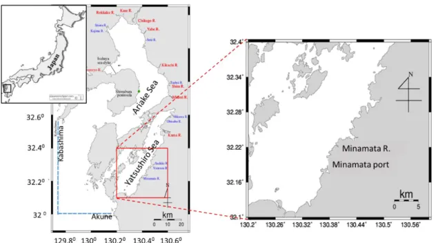
Figure 6.1. Measurement stations in Minamata Bay ... 91
Figure 6.2. Dendrogram for all data of SS particle size distribution ... 93
Figure 6.3. Relationship between the number of groups R and R
s... 95
Figure 6.4. Representative SS particle size distribution in each group (in case of 6 groups) ... 96
Figure 6.5. Relationship between SS particle size distribution pattern group and particulate THg concentration (mean±standard deviation) ... 97
Figure 6.6. Relationship between specific surface area of SS and particulate THg concentration for all data ... 98
Figure 6.7. Relationship between mean specific surface area of SS and mean
particulate THg concentration for 6 groups ... 99
1
Chapter 1
Introduction
1.1 Research Background
The environmental problem nowadays has become public awareness because it is occurring in many countries in the world. It degrades the quality of the environment and the life of organism living there. One of the problems is the water and air pollution by the excessive and untreated chemical compound disposal. The most tragic and enormous incident of the environmental pollution was the mercury problem in Minamata, Japan that occurred around 1956 which caused by the disposal of mercury by the chemical factory from 1932-1968 (Rajar et al., 2004; Balogh et al., 2015).
The Minamata incident exceeds 1,400 deaths later named “Minamata Disease” and
almost 40,000 people were suffered by the mercury intoxication and have been
identified to have partial symptoms of this disease (Minamata Disease Municipal
Museum, 2001; Japan Ministry of Environment, 2013). Methylmercury (MeHg), the
most toxic compound of mercury species was formed during the disposal and mostly
deposited in the sediment. This compound has contaminated the fish and other
organisms in the ocean and it ends up in the human body as it consumed (Zagar et al.,
2007). At that time the concentration of methylmercury in bottom sediment was
approximately 2,700 ppm (Akagi, 1995). A great number of MeHg if it compared with
the mercury regulation in Japan which only allow total mercury concentration 0.005
ppm for standard effluent and 0.0005 ppm for environmental quality standard according
to Environment Agency Notice No. 64 (September 1974) (Ministry of Environment,
2
2004). Later, the remediation project from 1977-1990 which removed the highly contaminated sediment to the shore has made the total mercury (THg) concentration in the bottom sediment around Minamata Bay reduced significantly to 8.85 ppm (Tomiyasu et al., 2006).
This kind of ‘disaster’ happens in other continents as well. In Canada, mercury pollution was also caused by a caustic soda factory and the methylmercury was produced through the methylation of the inorganic mercury contaminated the environment. Another evidence was found in Amazon River, Brazil in 1988 on some of the resident’s hair that contains mercury values exceed 100 ppm. The same incident with Minamata occurred in Jirin City, China, methylmercury flew out of a chemical complex into a river. In Africa and some of South East Asian countries, mercury was used for gold mining and most of the effluent were discharged to the river or sea directly. Moreover in Europe, such as Gulf of Trieste in Slovenia that contaminated by mercury from mercury mining area (Harada, 2000; Rajar, et al., 2004). Mercury polluted the land, air, and water environment. Many studies all over the world have proved that the mercury is transforming and cycling on the global mercury cycle.
Once mercury enters the environment, mercury can go through cycles between air, land, and water and it will be removed through burial in the deep ocean or lake sediments or through entrapment in stable mineral compounds. Mercury itself is a conservative compound, and it can change into different forms. The elemental Hg (Hg
0) as the Hg in the air, the inorganic Hg (Hg
2+) as the Hg in water and sediment, and methyl-mercury (MeHg) as organic mercury in water and sediment. Those mercury species can transform to each other forms under some conditions and MeHg is known as the toxic Hg which consumed by sea organism. On certain conditions, MeHg is easily formed from inorganic Hg by the certain bacteria, called methylation process and for the contrary is called demethylation process. MeHg is consumed by zooplankton and small organism, and it can lead to the biomagnification and bioaccumulation process, where the highest consumer, human, is the most severe contaminated by mercury (Zagar et al., 2007). Mercury in (sea)water is categorized into particulate and dissolved components.
Meanwhile in Minamata Bay, particulate THg concentration was higher than dissolved
one in seawater (Matsuyama et al.,2011).
3
Mercury cycle and transport along with the fate of its compound in water and atmosphere have been studied from years ago as there are many research papers about it. Numerical modeling and field measurement are the most-widely methods performed by the researchers. Begin with the first generation model applied in 1 dimensional (1D) river or the freshwater environment around 1980-1990. In early 2000, the second generation model was the 2D unsteady model which applied in the lake and only in the water column. This also contains the sediment-water and air-water exchange modules also the biogeochemical and food chain modules. The third generation model, after the year of 2000, has succeeded to do a simulation on the 3D unsteady model which contain hydrodynamic module combine with sediment and air-water exchange, also the biogeochemical module (Yano, 2010; Rajar et al., 2004; Zagar et al., 2007). However, the mercury cycle which related with biogeochemistry cycle has not fully represented in any model or simulation as the complexion of chemical and physical processes involved in it. Until recently, only one model existed that incorporated air, land, and water into a unified whole (UNEP, 2013).
By simulating the mercury fate in the water compartment, it is expected this method
can become a tools for estimating the mercury level in the water for past, present, and
future conditions in order to maintain the low concentration of Hg in Minamata Bay
and its surroundings. In Minamata, the mercury cycle and transport modeling have been
conducted by some researchers. Rajar et al. (2004) did the research about mercury
transport and mass-balance around Minamata, Yano et al. (2013 and 2014) did some
researches about sediment transport which contained mercury, did the in-situ
measurement in Minamata Bay for 15 years, also laboratory experiment of methylation
process. They also estimated the relationship between SS grain size distribution with
the THg concentration, considering the particulate form of Hg in Minamata Bay is
higher than dissolved one. However, the simulation of mercury transport in the
sediment was done in a coarse grid where Minamata Bay is not clearly plotted. In
addition, the relation about suspended solid (SS) particle size distribution and total
particle Hg (THg) concentration is not clear yet. Therefore, the development model
which includes refine grid for the simulation and also better parameter values for
4
simulating the particulate mercury fate in Minamata Bay and the evaluation of SS grain size distribution and THg concentration will be presented in this research.
1.2 Research Problems
The investigation of mercury fate in Minamata Bay has already begun since long time ago. Until now, our research team still do the measuring of Hg in the bay for maintaining its Hg fate after the incident in 1956. Many studies about mercury fate and distribution in Minamata have already been done, but most of the simulation still use assumptions for the parameter because of insufficient data and information. Yano et al.
(2014) have done a sediment transport simulation containing Hg in Minamata Bay and the results were validated with field measurement by Rifardi et al. (1998). However, the simulation was used many assumptions and a coarse grid where the bay was not detail described.
In addition, the effect of dredging and reclamation in the bay also has to be investigated, in order to see its effectiveness. Because it is expected that there was still a small trace of Hg in which remain deposited in the bay. Furthermore, the reclamation wall that has been built for 30-40 years ago will deteriorate and may threaten the life surrounding the bay. The prediction of the incident could be one of the solutions to prevent bigger negative impact for the environment. The precise simulation data of the mercury transport incident need to be calculated in order to get a better result.
The relation between particulate total mercury and SS grain size distribution also has
to be re-evaluated because previous studies about it (Yano et al., 2013) was using
subjective method in determining the group of SS. This evaluation is necessary for
simulating sediment transport which contain particulate mercury in future works.
5
1.3 Research Objectives
The main objective of this work is to simulate the mercury transport in sediment, namely particulate mercury using finer grid and by the improvement, other simulations are been conducted, such as the simulation of before and after reclamation project and simulation of the damaged of reclamation wall. In order to get better and more actual description of mercury concentration in suspended solid and sediment around Minamata Bay, evaluation of SS particle size distribution and particulate total Hg are also been conducted. The details purposes of this thesis are presented in these following points:
To do simulation of mercury distribution especially in sediment from Minamata to Yatsushiro Sea by using a finer grid,
To compare how the mercury transport occur in before and after reclamation project,
To do simulation if the reclamation wall in Minamata Bay is damaged and releasing high contaminated sediment by mercury to the bay,
To evaluate relationship between SS particle size distribution and particulate total Hg concentration in Minamata Bay, and
To validate the simulation result by comparing it with real measurement data.
6
1.4 Scope of the Study
The concerning mercury dynamics in this works are in aquatic and sediment environment, so this research only considers the process in water body and sediment and neglecting the atmospheric aspect. Furthermore, this research focuses on simulation by using improve grid, parameter, and other data of mercury fate in sediment and suspended solid in water.
The most dangerous Hg compound, MeHg, is mostly deposited as sediment in the sea
bottom. By that consideration, the MeHg is simulated as sediment-mud due to the lack
of data source because there is no actual and complete data of MeHg concentration in
Minamata Bay sediment. This method is used to see the pattern of sediment transport
which may contain Hg that can be distributed to outside the bay. Furthermore, the
evaluation of particulate THg concentration and SS grain size distribution is using data
from field measurement which conducted by Yano et al. since 2006.
7
1.5 Overview of the Thesis
This thesis is consist of literature review and some research topics which have been published in proceedings and a journal. The total chapters of this thesis are seven chapters and described as follow:
CHAPTER 1 contains the research background, research problem, research objective, the scope of the study, and overview of the thesis.
CHAPTER 2 is a literature review which explains about mercury dynamics in the global environment include its source, mercury budget, mercury cycle, and also mercury problems. The explanation of mercury problem includes a brief description mercury contamination in the world and main explanation about mercury contamination in Minamata Bay. Furthermore, the explanation of mercury transport in bottom sediment, such as the numerical model and also governing equations are presented in this chapter.
CHAPTER 3 presents a numerical simulation of fine sediment transport in Minamata Bay using a variable grid. In this chapter, the new grid system of sediment transport simulation is introduced. The model, variable grid system, numerical explanation, input parameter, and also the result and discussion are also explained in this chapter. The results compare bottom sediment transport pattern by previous and the new grid system in barotropic and baroclinic conditions.
CHAPTER 4 discusses the impact of reclamation project on mercury-contaminated sediment transport from Minamata Bay into the Yatsushiro Sea. It includes the model description, validation of simulations, result and discussion which explain about the hydrodynamic condition and also bottom sediment transport in before and after reclamation projects.
CHAPTER 5 describes numerical simulation of sediment transport and suspended solid
(SS) distribution due to the damage of reclamation wall in Minamata Bay. This
simulation shows how the suspended solid and bottom sediment distribution in
Minamata Bay when the reclamation wall which had been built around 30 years ago
collapse, and releasing the high contaminated sediment to the water environment. This
8
chapter also includes numerical modeling which explains about its computational domain and grid, the calculation method, boundary condition, input parameter, and scenarios. The results compare the SS distribution when the south part and north part of the wall collapse and also compare when the incident happen in barotropic and baroclinic conditions.
CHAPTER 6 evaluates the relation between particulate total mercury in seawater and suspended solid particle size distribution in Minamata Bay. Here, the new cluster method of SS data grouping is proposed and evaluated the statistical significance between SS particle size distribution pattern group and particulate THg concentration.
The result shows a regression formula which can estimate the concentration of particulate THg from SS particle size distribution.
CHAPTER 7 is the conclusion and recommendation. This chapter summarizes the
whole research works in this thesis and also gives some suggestions and
recommendation for future works.
9
References
Akagi, H. (1995). Methylmercury pollution-Minamata Bay after Minamata Disease outbreak and the latest problems in the foreign countries, Medicina Philosophica, 14(8), pp. 597-604. (In Japanese)
Balogh, S. J., Tsz-Ki Tsui, M., Blum, J.D., Matsuyama, A., Woerndle, G.E., Yano, S.
and Tada. A. (2015). Tracking the fate of mercury in the fish and bottom sediments of Minamata Bay, Japan, using stable mercury isotopes, Environ.
Sci. Technol., 49(9), pp.5399–5406.
Harada, M. (2000). Minamata Disease and the Mercury Pollution of the Globe, Retrieved from http://www.einap.org/envdis/Minamata.html
Matsuyama, A., Eguchi, T., Sonoda, I., Tada, A., Yano, S., Tai, A., Marumoto, K., Tomiyasu, T., and Akagi, H. (2011). Mercury Speciation in the Water of Minamata Bay, Japan, Water, Air and Soil Pollution, 218, 399-412.
Ministry of Environment, Japan. (2004). Mercury Analysis Manual. Environmental Health and Safety Division, Environmental Health Department. Ministry of the Environment, Japan.
Rajar, R., Zagar, D., Cetina, M., Akagi, H., Yano, S., Tomiyasu, T. and Horvat, M.
(2004). Application of three-dimensional mercury cycling model to coastal seas, Ecological Modeling, 171, pp.139-155.
Tomiyasu, T., Matsuyama, A., Egushi, T., Fuchigami, Y., Oki, K., Horvat, M., Rajar, R. and Akagi, H. (2006). Spatial variations of mercury in sediment of Minamata Bay, Japan, Sci. Total Environ., 369, pp.283- 290.
United Nations Environment Programme (UNEP). (2013). Global Mercury Assessment 2013: Sources, Emissions, Releases and Environmental Transport. UNEP Chemicals Branch, Geneva, Switzerland: 1–42at
Yano, S. (2010). On development of a numerical model for understanding mercury
10
behaviors in Minamata Bay. Proceeding of NIMD (National Institute for Minamata Disease) Forum 2010 : Environmental cycling of methylmercury in aquatic systems.
Yano, S., Hisano, A., Kawase, H., Matsuyama, A., Tai, A., Riogilang, H., Tada, A., and Sonoda, I. (2013). Relationship between Particulate Total-Mercury in Seawater and Grain Size Distribution of Suspended Solids in Minamata Bay.
Journal JSCE B2, 69(2), pp.I_1081-I_1085. (In Japanese with English abstract)
Yano, S., Kawase, H., Hisano, A., Riogilang, H., Tada, T. and Matsuyama, A. (2014).
The effect of salinity stratification on sediment transport in Minamata Bay, Proceeding of the 19
thIAHR-APD Congress 2014, in USB memory.
Zagar, D., A. Knap, J.J. Warwick, R. Rajar and M. Horvat. (2007). Modelling of
mercury transport and transformations in the water compartment of the
Mediterranean Sea, Marine Chemistry, 107, pp.64–88.
11
Chapter 2
Mercury Dynamics in Natural Environment
2.1 Mercury in Global Environment
The rapid growth of industry since the beginning of modernization era is followed by
the increasing of problem awareness caused by it. One of them is the heavy metal
pollution problem, especially the mercury compound. Mercury is known as a heavy
metal which used for industrial purposes. However, behind its usefulness, just like other
heavy metals, mercury is very dangerous, moreover if it enters the human and other
organism’s body. Mercury is released to the environment from natural sources and
processes and also as a result of human activities. Mercury can go through a cycles
between air, land, and water once it has entered into the natural environment, and it will
be removed through burial in deep ocean or lake sediments or through entrapment in
stable mineral compounds. However, after it is buried in sediment, actually mercury
can be re-suspended by physical and chemical process, such as currents or wave and
bacteria activities. Especially the methylmercury (MeHg), the most toxic and
bioaccumulative form of mercury, which presents the greatest health risk to humans
and wildlife is mainly formed in aquatic environments through natural microbial
processes.
12
2.1.1 Source of mercury emission to air and water
The sources of mercury emission can be divided into three sources, first is natural sources, second is anthropogenic sources, and last is the re-emission/re-mobilization of it. Basically, mercury can be found throughout the world as a natural element. It is contained in some minerals, such as cinnabar, an ore mined to produce mercury. Then, the anthropogenic is a human activity such as mining and burning of coal which also has increased the mobility of mercury in the environment. In addition the mercury itself will go through the re-emission and re-mobilization (UNEP, 2013).
Natural process of mercury emission, namely such as the mercury-containing rocks which experiences weathering continuously will allows mercury to escape to air and to be washed into lakes and rivers. Furthermore, eruption of volcano can emit and release mercury and geothermal activity can take mercury from underground and emit it to the air and release it to the deep ocean. This natural emission of mercury contributes around 10% of the estimated mercury in the atmosphere from all sources.
Mercury emission by human activity has already begun since 1800 when the revolution of industry occurred. At that time, coal burning, mining, cement production, and oil refining have increased the mercury emission to atmosphere and release to water environment. Moreover, the emission can be caused by wastes from consumer products such as batteries, paints, switches, electronic devices, thermometers, blood-pressure gauges, fluorescent lamps, pesticides, fungicides, medicines, and cosmetics. In addition, mercury is also used in a number of industrial processes. A major industrial use is in the chlor-alkali industry where mercury-cell technology may be used in the production of chlorine and caustic soda. Mercury is also used as a catalyst in the production of vinyl chloride monomer (VCM) from acetylene, mainly in China. This anthropogenic sources of mercury contributes for about 30% of the total amount of mercury entering the atmosphere each year and 50% of the atmosphere emission is from Asia region, namely East and Southeast Asia (UNEP, 2013).
The last source of mercury emission is the re-emission and re-mobilization processes
of mercury. It contributes around 60% of mercury emission to the air. Re-emission is a
13
result of natural processes that convert inorganic and organic forms of mercury to elemental mercury, which is volatile and therefore readily returns to the air. Mercury deposited to plant surfaces can be re-emitted during forest fires or biomass burning.
Mercury may be deposited and re-emitted many times as it cycles through the environment. In the aquatic environment, re-mobilization of mercury occurs when mercury deposited on and accumulated in soils or sediments is re-mobilized by, for example, rain or floods that cause the mercury to enter or re-enter the aquatic system.
Resuspension of aquatic sediments due to wave action or storm events is an additional way for mercury to re-enter the aquatic ecosystems.
2.1.2 Global mercury budget
The presence of mercury in the land, air, and ocean is in unsteady state and it can change over between those 3 reservoirs. The model of mercury budget in the air, land and atmosphere has been presented by Selin et al. (2008) and modified in Selin (2009).
Figure 2.1 is the result of global 3D land-ocean-atmosphere model for mercury (Selin, 2009). The black line is indicated natural fluxes of mercury involves atmospheric transport, deposition to land and ocean, and re-volatilization. The red line is the anthropogenic sources, and the red-black dotted line is the combination of both natural and anthropogenic sources, all number unit are in Megagram (Mg)/year or ton/year.
In preindustrial time, the anthropogenic and biomass emission are not included yet, the
budgets are written by black color (Figure 2.1). At the present day, the anthropogenic
and biomass burning emission are included due to the industrial activities which use
mercury. Human contribution of mercury emission to the air and ocean gives significant
number of the mercury amount in the atmosphere and ocean. The most dominant source
is the anthropogenic sources that has made the atmosphere budget increases as well as
the deposition to land and ocean, and made mercury budget in surface ocean also
increases. The ultimate sink of mercury is burial to the deep-ocean sediments, which
occurs very slowly. The overall (e-folding) lifetime of mercury in the combined
14
atmosphere-ocean-terrestrial system against transfer to the sediments is 3,000 years (Selin, 2009).
Figure 2.1. Global Mercury Budget. [Unit: Mg/year]
Reprinted from “Global Biogeochemical Cycling of Mercury : A Review,” by Selin, N.E, 2009, Annu.
Rev. Environ. Resour, 34, p. 43-63. Copyright 2009 by Annual Reviews
The geogenic, antrophogenic, biomass burning, soil and vegetation contribute for
mercury emission to the atmosphere resulting around 5,600 Mg/year mercury stays in
the atmosphere. In soil, the mercury amount is around 1.15x10
6Mg/year, also there is
small fraction that released from land to ocean through river and ground water. Rivers
are estimated to carry more than 2,800 tons of mercury each year, but only about 380
tons of this is transported offshore. The rest is trapped by particles in estuaries.
15
Groundwater and re-mobilization from sediments provide 100-800 tons of mercury to
the oceans each year (UNEP, 2013). From atmosphere, the elemental mercury Hg(0)
and particulate mercury Hg(II)P will be deposited again to the land and ocean, where
the ocean receives more than land. In ocean the mercury budget is divided in 3 area,
first is the surface which directly interact with atmosphere deposits around 7,000
Mg/year mercury. Then it will through exchange with deep ocean and it deposited
around 350,000 Mg/year. In the end it will be buried in very slow process to the deep-
ocean sediment which deposits 3x10
11Mg/year mercury (Selin et al., 2008; Selin 2009).
16
2.2 Mercury Cycle
Mercury is a conservative compound, the compound that can last long in water body before finally settles or absorbed by the various physical and chemical reactions in water. Mercury can change into different forms, the elemental Hg (Hg
0) as the Hg in air, the inorganic Hg (Hg
2+) as the Hg in water and sediment, and mono methyl mercury (MeHg) as organic mercury in water and sediment (Zagar et al.,2007). Those mercury species can transform to each other forms under some conditions. The mercury transformation is included in biogeochemical cycle. Biogeochemical cycle is a pathway by which a chemical substance moves through both biotic (biosphere) and abiotic (lithosphere, atmosphere, and hydrosphere) compartments of the earth (Wikipedia, 2017). Figure 2.2 shows the mechanism of biogeochemical cycle of mercury.
Figure 2.2. Biogeochemical cycle of Mercury.
Reprinted from Mercury inventory for New Zealand: 2008, Retrieved February 20, 2017, from http://www.mfe.govt.nz/sites/default/files/pubs/figure-i-3.jpg. Copyright 2009 by Ministry for the Environment New Zealand.
There are 12 processes that change mercury species in the air, water, and soil or
sediment. The emission of mercury occurs when the elemental Hg is released to the
17
atmosphere originating from volcanoes and mining industries. Then it is deposited to the land and water area, which then finally flows to the sea. The landfills and farming activities also play a role in this process, where mercury and other chemicals are absorbed into the ground and then flow into the river and end up in the sea. After that, the mercury is deposited as sediment in sea bottom mostly as MeHg and evaporated to the air as elemental Hg.
The transformation of each mercury species occurs in water environment and soil. The elemental mercury can transform become inorganic mercury by oxidation process, and reduction process for the contrary. The inorganic Hg can transform into MeHg by the help of certain bacteria, called methylation process and for the contrary is called demethylation process. MeHg is consumed by zooplankton and small organism, and it can lead to the biomagnification process, where the highest consumer, human, is the most severe contaminated by mercury. The organic mercury including MeHg can be absorbed as a sediment and will be re-suspended and desorption become particulate form in water bodies. Those transformation processes also occur in soil environment.
All of the processes is repeated and form a cycle, called mercury cycle.
1. Mercury in the air
As mention above, most mercury in the air is in elemental forms, although actually there are three primary forms, gaseous elemental form (Hg
0), gaseous oxidized mercury and particulate mercury. The oxidized and particulate one are more ready to move to the water and land and it will be re-emitted again to the air when it has been converted to gaseous elemental mercury again. Sunlight is the dominant factor of oxidation and reduction process, and also in some degree, the temperature and biological interaction are involved (UNEP, 2013).
2. Mercury in the aquatic environment
In fresh waters and marine environment, the dominant mercury is inorganic Hg both
in dissolved and particulate form, whereas the dissolved gaseous elemental mercury
is less than 30% of total Hg in water. This inorganic Hg can change into
methylmercury (MeHg), the toxic species of Hg that can concentrates in animal and
human body, and it reach 30% of total mercury. In freshwater and coastal region,
18
the conversion of inorganic Hg to methylmercury (methylation process) primarily occurs in sediments. Meanwhile in the open ocean the methylation usually occur between 200-1000m in the water column (Zagar et al., 2007; UNEP, 2013). In general, from the analysis of relation Hg in water, there is a positive correlation Hg with temperature and BOD, and negative correlation Hg with DO, pH, and salinity (Menon and Mahajan, 2010). The occurrence and migration of different mercury species in water environment depends also to a great degree on the red-ox conditions and the content of dissolved organic carbon (DOC) (Boszke et al., 2002).
The nutrient also affected the mercury dynamics in seawater, increases in nutrient loading alter coastal ecosystems in ways that should change the transport, transformations and fate of Hg (Driscoll et al., 2012). MeHg formation rate increased with nutrient loading only for HgII tracers with a high availability for methylation. Tracers with low availability did not respond significantly to nutrient loading (Nguyen et al., 2016).
Mercury output from aquatic systems are in two ways. First when inorganic mercury is reduced to elemental mercury then it can be re-emitted to the atmosphere.
Second when inorganic mercury binds to particulates in water, it can settle out rapidly and be buried in sediments. Deep burial in ocean sediments is one of the major pathways by which mercury is removed from the biologically active environment (UNEP, 2013).
3. Mercury in sediment
As mention above, the particulate forms of inorganic mercury and also
methylmercury can settle as sediment in bottom layer. In sediment of coastal
environment, mercury mostly found as MeHg compound although the source of it
is not yet clearly understood (Han et al., 2010). Under normal conditions, around
5% of inorganic mercury may change to MeHg compound (methylation process)
(Yano et al., 2013). That process mostly occurs in water column and depends on
many factors, such as salinity, temperature, pH, DOC, nutrients, and also the
existence of certain bacteria. Meanwhile in sediment, which do not contain salt,
mercury absorption depends on the pH (Boszke et al., 2003). Heavy metal contents
in total sediment are closely linked with the percentage of the <16
m fraction, or
19
the other words, it can be classified as silt or mud in bottom sediment (Barghigiani et al., 1996).
Mercury output from sediment also can be divided in two ways, first is when the
resuspension occur which could lift sediment to the water column and second way
is through the deep burial in bottom sediment.
20
2.3 Mercury Problems
2.3.1 Mercury contamination in the world
Mercury contamination has become an awareness for global society nowadays, although actually the mercury contamination to environment had already begun long time ago. As we know, the Minamata disease in Japan happened in 1956, and followed by the second Minamata disease in Niigata, Japan in 1965, both were caused by methyl mercury contamination in the aquatic environment that used by factories for producing acetaldehyde.
These problems also occurred in another countries in the world. In America, Canada and Brazil were struggled with mercury pollution. Similar case was found in Canada where a caustic soda factory produced the methylmercury compound through the methylation of the inorganic mercury contaminated the environment. In Amazon River, Brazil, some of the resident’s hair were contained mercury which exceed 100 ppm. In Asia, China and Southeast Asian countries such as Indonesia used mercury for illegal gold mining and the effluent were discharged to the river or sea directly (Harada, 2000;
Ismawati, 2012). In Iraq, ethylmercury and methylmercury poisonings were following
by the consumption seed grain that had been treated with fungicides containing these
alkylmercury compound. These incidents afflicted more than 6,000 people and resulted
in 400 deaths (UNEP, 2002). In other cases also found in Africa, most of gold mining
or chemical factory used mercury in their process. In Europe, Rajar et al. (2004)
reported that in the Gulf of Trieste in Italy and Slovenia was contaminated by mercury
from mercury mining area. The mercury polluted the land, air, and water environment.
21
2.3.2 Mercury contamination in Minamata Bay 2.3.2.1 Minamata disease outbreak
In Minamata, mercury contamination was caused by production of acetaldehyde from Chisso factory. The Chisso factory used mercuric sulfate as catalyst in the process of manufacturing acetaldehyde. In this process, some of mercuric sulfate turned into methylmercury (Kashiranui, 2014). The formation of methylmercury compound is shown in Figure 2.3. This MeHg compound also is a change form of inorganic mercury compound mercury(II)b oxide (HgO) which was disposed to Minamata Bay without adequate treatment by the factory from 1932-1968 (Balogh et al., 2015).
Figure 2.3. Methylmercury formation in Chisso Factory, Minamata.
Reprinted from Preparatory Study for Minamata Field Work, Retrieved May 19, 2015, from http://www.mkplan.org/download/downloadfiles/kisogakusyuu_en2014.pdf. Copyright 2014 by Kanshiranui Planning General Incorporated Association.
22
Methylmercury (MeHg) compound which mostly deposited in seabed as sediment (Zagar et al., 2007) can be consumed by zooplankton, then this contaminated zooplankton is consumed by small fishes, then they are consumed by big fishes and the last consumer, human (Figure 2.4). Hg through a biomagnification and bioaccumulation processes in the food chain is resulting human as the most severe contamination by mercury.
Figure 2.4. Mercury biomagnification and bioaccumulation mechanism in Minamata
Reprinted from “History and current state of waste management in Japan ,” pamphlet by Ministry of the Environment, 2014. Copyright 2014 by Japan Environmental Sanitation Center.