Navier-Stokes 方程式に対する時間2次精度特性曲線有限要素スキームの安定性(数値シミュレーションを支える応用数理)

(1)

Navier-Stokes

方程式に対する時間

2 次精度特性曲線

有限要素スキームの安定性

Stability of

a characteristic

finite element

scheme

of

second order in

time increment

for the

Navier-Stokes

equations

九州大学大学院数理学研究院

野津裕史

(Hirofumi NOTSU)*

田端正久

(Masahisa

TABATA)\dagger

Faculty

of Mathematics,

Kyushu

University

1 Introduction

Let $\Omega$be abounded domain in

$\mathbb{R}^{d}(d=2,3)$ and $T$beapositiveconstant. WeconsIderthe problem governed by the nonstationary Navier-Stokes equations subject to the Dirichlet boundary conditions; find $(u,p)$ : $\Omega x(0,T)arrow \mathbb{R}^{d}x\mathbb{R}$such that

$\{\begin{array}{ll}\frac{\partial u}{\theta t}+(u\cdot\nabla)u-\nabla(2\nu D(u))+\nabla p=f in \Omega x(0,T),\nabla\cdot u=0 in \Omega x(0,T),u=g on \Gamma x(0,T),u=u^{0} in \Omega, at t=0,\end{array}$ (1)

where

$u$ is the velocity, $p$ is the

pressure,

$f$ is

an

exterior force, $g$ is

a

boundary velocity,

$u^{0}$ is

an

initial velocity,

$\nu(>0)$ is

a

viscosity, $\Gamma\equiv\partial\Omega$, and $D(u)$ is the strain-rate tensor

defined by

$D_{ij}(u) \equiv\frac{1}{2}(\frac{\partial u_{t}}{\partial x_{j}}+\frac{\partial u_{j}}{\partial x_{1}})$

.

A $secondorder-\ddagger n$-time characteristic finite element scheme for convection-diffusion

problems had been developed in [2], where they had proved stability and

convergence

theorems. Using theiridea,

we

have developed

a

second ordercharacteristic finiteelement

scheme [1] for (1). Ourscheme is thecombination of

a

second-order-in-time characteristic

finite element scheme and the

ffist-order-in-time

characteristic finite element scheme (see

Figure 1). _{The scheme has such advantages that it} _is_{of second} _order _in $\Delta t$ and

that

the

matrices

are

symmetric. The combined scheme is stable

even

for high Reynolds number

problems. Inthispaper

we

considerthe stability. Thecontentsofthe paper

are

as

follows.

’E-mail: notsuOmath.kyushu-u.ac.jp

$\dagger_{E}$

(2)

$...arrow(_{p_{h}^{n-1}}^{u_{h}^{n-1}})arrow^{\Delta t_{0}=O(\Delta t)Secondorder}(\begin{array}{l}u_{h}^{n-\alpha}p_{h}^{n-\alpha}\end{array})arrow^{\Delta t_{1}=O(\Delta t^{2})Firstorder}(\begin{array}{l}u_{h}^{n}p_{h}^{n}\end{array})arrow\cdots$

Figure 1: Time evolution ofthe scheme

We introduce the scheme in Section 2 and present a sufficient condition for the scheme

to be stable in Section 3. In the last section

we

check the condition numerically in

an

example and solve

a

cavity flow problem with high Reynolds numbers.

We

use

the function spaces $L^{2}(\Omega)$ and $W^{1,\infty}(\Omega)$

.

For

any

normed

space

$X$

we

use

the

notation $\Vert\cdot\Vert_{X}$

to

represent the

X-norm.

We omit $\Omega$ in the notations

of

norms, and

use

$\Vert\cdot||$ to show the $L^{2}$

-norms

$\Vert\cdot\Vert_{L^{2}},$ $\Vert\cdot\Vert_{(L^{2})^{i}},$ $\Vert\cdot\Vert_{(L^{2})^{dxi}}$

.

2 A

second order

characteristic finite element scheme

For time increments $\Delta t$

,

\Deltaが and velocities

$u,$ $v$ : $\Omegaarrow \mathbb{R}^{d}$,

we

define $X_{1}(u, \Delta t)$ and

$X_{2}(u,v, \Delta t’, \Delta t)$ by

$X_{1}(u, \Delta t)(x)\equiv x-u(x)\Delta t$

,

$X_{2}(u, v, \Delta t’, \Delta t)(x)\cong x-\{(1+\frac{\Delta t}{2\Delta t})u(x-u(x)\Delta t’)-\frac{\Delta t}{2\Delta t}v(x-u(x)(\Delta t’+\Delta t..\}\Delta t’$

,

respectively. The $X_{1}(i=1,2)$

are

used for the i-th order approximate values of_upwind

points. For

a

function $\psi$

over

$\Omega x(0,T)$,

we

set $\psi^{n}\equiv\psi(\cdot, t^{n})$, where $t^{n}$ is defined by

$t^{n}\equiv n\Delta t$

.

The symbol $\circ$

means

the composition of functions,

$(\psi^{n}\circ X)(x)\equiv\psi^{\mathfrak{n}}(X(x))$

.

Let $\mathcal{T}_{h}=\{K\}$ be

a

triangulation of$\Omega$

.

We define $\Omega_{h}$ by

$\Omega_{h}\equiv int\cup\{K;K\in \mathcal{T}_{h}\}$

and$\Gamma_{h}\equiv\partial\Omega_{h}$

.

Let$\Delta t$be

a

timeincrement, and_{$N_{0}$} be

a

positiveinteger.

We

set

$\alpha\equiv 1/N_{0}$

,

$\Delta t_{0}\equiv(1-\alpha)\Delta t$

and

$\Delta t_{1}\equiv\alpha\Delta t$

.

We

define A

by

$A\equiv\{n\in \mathbb{R};n=m\alpha, m\in N, 1\leq m\leq N_{0}\}\cup\{n\in \mathbb{R};n\in N\cup(N-\alpha), 1\leq n\leq N_{T}\}$

and set $\Lambda_{0}\equiv\Lambda\cup\{0\}$, where $N_{T}\equiv[T/\Delta t]$

.

In the following definitions

we

use

the

same

notation $(\cdot, \cdot)$ to represent the $L^{2}(\Omega_{h})$-inner products in the scalar- and vector-valued

function spaces. Suppose $\{u_{h}^{n}\}_{n\in\Lambda_{0}}\subset H^{1}(\Omega_{h})^{d},$ $\{p_{h}^{\mathfrak{n}}\}_{\mathfrak{n}\in\Lambda}\subset H^{1}(\Omega_{h})$ and $f\in C^{0}(L^{2}(\Omega_{h})^{d})$

be given. We definelinearforms$\mathcal{A}_{0h}^{\mathfrak{n}-\alpha}(u_{h},p_{h}),$$\mathcal{A}_{1h}^{n}(u_{h},p_{h}),$$P_{0h}^{1-\alpha}(f, u_{h}),$$P_{1h}^{\iota}f$

on

$H_{0}^{1}(\Omega_{h})^{d}$

and $\mathcal{B}_{h}^{\mathfrak{n}}u_{h}$

on

$L_{0}^{2}(\Omega_{h})$

as

follows:

$\langle A_{h}^{n-\alpha}(u_{h},p_{h}), v_{h}\rangle\equiv(\frac{u_{h}^{n-\alpha}-u_{h}^{n-1}oX_{2}(u_{h}^{n-1},u_{h}^{n-2},\Delta t_{0},\Delta t)}{\Delta t_{0}},$_{$v_{h})$}

$+\nu(D(u_{h}^{n-a})+D(u_{h}^{n-1})\circ X_{1}(u_{h}^{n-1}, \Delta t_{0}),$$D(v_{h}))+ \nu\Delta t_{0}\sum_{t_{\dot{\theta}},k=1}^{d}(D_{ij}(u_{h}^{n-1})u_{hk,j}^{n-1},v_{hi,k})$

(3)

$\langle \mathcal{A}_{1h}^{n}(u_{h},p_{h}), v_{h}\rangle\equiv(\frac{u_{h}^{n}-u_{h}^{n-\alpha}\circ X_{1}(u_{h}^{n-\alpha},\Delta t_{1})}{\Delta t_{1}},$ _{$v_{h})+2\nu(D(u_{h}^{n}),$} _{$D(v_{h}))-(\nabla\cdot v_{h},p_{h}^{n})$},

$\langle \mathcal{F}_{0h}^{n-\alpha}(f, u_{h}), v_{h}\rangle\equiv\frac{1}{2}(f^{n-\alpha}+f^{n-1}\circ X_{1}(u_{h}^{n-1}, \Delta t_{0}),$_{$v_{h})$}, _{$\langle F_{1h}^{t}f, v_{h}\rangle\equiv(f^{n}, v_{h})$},

$\langle \mathcal{B}_{h}^{n}u_{h}, q_{h}\rangle\equiv(\nabla\cdot u_{h}^{n}, q_{h})$

.

We set finite element spaces

$X_{h}\equiv\{v_{h}\in C^{0}(\overline{\Omega}_{h})^{d};v_{h}|_{K}\in P_{2}(K)^{d},$ $\forall_{K\}}$

$V_{h}(g)\equiv\{v_{h}\in X_{h};v_{h}(P)=g(P)(node P.\in\Gamma_{h})\}$, $V_{h}\equiv V_{h}(0)$, $Q_{h}\equiv\{q_{h}\in C^{0}(\overline{\Omega}_{h});q_{h}|_{K}\in P_{1}(K),$ _{$\forall_{K}\int_{\Omega_{h}}q_{h}dx=0\}$}

.

Forthe given function $f$ the notation $f_{h}(\cdot, t)$

means

$\Pi_{h}f(\cdot, t)$, where $\Pi_{h}$ : $C^{0}(\overline{\Omega}_{h})^{d}arrow X_{h}$

is the interpolation operator.

A second order

characteristic finite element

approximation to problem (1) is the

fol-lowing; find $\{(u_{h}^{n}, p_{h}^{\mathfrak{n}})\in V_{h}(g^{n})xQ_{h};n\in\Lambda\}$such that

general stage:

$\{\begin{array}{ll}A_{0h}^{n-\alpha}(u_{h},p_{h})=\mathcal{F}_{0h}^{n-\alpha}(f_{h}, u_{h}) in V_{\hslash},\mathcal{B}_{h}^{n-\alpha}u_{h}=0 in Q_{h}’,\end{array}$ (2a)

$\{\begin{array}{ll}A_{1h}^{n}(u_{h},p_{h})=\mathcal{F}_{1h}^{m}f_{h} In V_{h}’,\mathcal{B}_{h}^{n}u_{h}=0 in Q_{h}’,\end{array}$ (2b)

$(n=2, \cdots N_{T})$,

initial stage:

$\{\begin{array}{ll}\mathcal{A}_{1h}^{m\alpha}(u_{h},p_{h})=F_{1h}^{m\alpha}f_{h} in V_{h)}’\mathcal{B}_{h}^{m\alpha}u_{h}=0 in Q_{h}’,u_{h}^{0}=\Pi_{h}u^{0}, \end{array}$ (2c)

$(m=1, \cdots N_{0})$

.

We find $(u_{h}^{n-\alpha},p_{h}^{n-\alpha})hom(2a)$ and find $(u_{h}^{n},p_{h}^{n})$ ffom (2b). The absence of $(u_{h}^{1}, p_{h}^{1})$ is

covered by (2c). (2a) is

a

second order scheme in $\Delta t_{0}$, and (2b) and (2c)

are

first order

schemes in $\Delta t_{1}$

.

If

we

set _{$\Delta t_{0}=O(\Delta t)$} and _{$\Delta t_{1}=O(\Delta t^{2})$}, the scheme (2) is of second

order in $\Delta t$

.

3 Stability of the scheme

In this section

we

present

a

proposition

on

the stability of the scheme. Thosehypotheses

are

checked numericaUyin

Section

4.

For

a

givenseries$\{w^{n}\}_{n\in\Lambda_{0}}$in

a

normedspace$X$,

we

introduce

norms-

$\Vert\cdot||\iota\infty(x),$ $||\cdot\Vert_{l^{2}(X)}$,

$\Vert\cdot\Vert_{l_{\Lambda}^{2}(X)}$ defined by

$||w||_{l(X)} \infty\equiv\max_{\mathfrak{n}\in\Lambda_{0}}||w^{n}||_{X}$,

(4)

$||w \Vert_{l_{A}^{2}(X)}\equiv\{\Delta t_{1}\sum_{m=1}^{N_{0}}\Vert w^{m\alpha}||_{X}^{2}+\sum_{n=2}^{N_{T}}(\Delta t_{0}\Vert w^{n-\alpha}||_{X}^{2}+\Delta t_{1}||w^{n}\Vert_{X}^{2})\}^{1/2}$

.

Hypothesis 1. There exists

constants

$M_{1},$ $M_{2},$ $c_{1}$ and $c_{2}$ independent

of

$\Delta t,$ $\alpha$ and $h$

such that

$\{\begin{array}{l}||u_{h}\Vert_{l\infty((W^{1,\infty})^{d})}\leq M_{1}X_{1}(u_{h}^{(m-1)\alpha}, \Delta t_{1})(\Omega)\subset\Omega(m=1, \cdots N_{0}),X_{1}(u_{h}^{n-\alpha}, \Delta t_{1})(\Omega)\subset\Omega X_{1}(u_{h}^{n-1}, \Delta t_{0})(\Omega)\subset\Omega,X_{2}(u_{h}^{\mathfrak{n}-1},u_{h}^{n-2}, \Delta t_{0})(\Omega)\subset\Omega(n=2, \cdots N_{T})\forall_{n}(n=2, \cdots N_{T}),\nu\Vert D(u_{h}^{n})\Vert^{2}\leq\nu(1+c_{1}\Delta t_{0})||D(u_{h}^{n-\alpha})\Vert^{2}+c_{2}||f_{h}^{\mathfrak{n}}\Vert^{2}\Vert\nabla p_{h}\Vert_{l^{2}((L^{l})^{d})}\leq M_{2}\end{array}$

Proposition 1. Let $(u_{h},p_{h})$ be the solution

of

(2) with $g=0$

.

Suppose that Hypothesis 1

holds. Then there exists a positive constant $C$ independent

of

$\Delta t,$ $\alpha$ and $h$ such that

1I

$u_{h}\Vert_{\iota\infty_{t(L^{2})^{\ell})}}+\sqrt{\nu\Delta t_{0}}\Vert D(u_{h})\Vert_{l((L^{2})^{dxd})}\infty$

$\leq C\{\Vert u_{h}^{0}||+\sqrt{\nu\Delta t}\Vert D(u_{h}^{0})\Vert+\Vert\nabla p_{h}\Vert_{l^{2}((L^{2})^{d})}+\Vert f_{\hslash}\Vert_{l_{\Lambda}^{2}((L^{2})^{d})}\}$

.

4 Numerical

results

In this section

we

show numerical results in $d=2$ with $P2/P1$ element. _{In [4] it} _is

remarked that much attention should be paidto numerical integration ofcomposite

func-tions. We used

a

numerical integration formula of degree five

on

each triangle [3].

For

a

number $N\in N$

we

set $\Delta t\equiv 1/N$ and $N_{0}\equiv N+1$, i.e.,

$\Delta t=\frac{1}{N}$, $\Delta t_{0}=\frac{1}{N+1}$

,

_{$\Delta t_{1}=\frac{1}{N(N+1)}$}

.

(3)

Since

it holds that

$\Delta t_{0}=O(\Delta t),$ $\Delta t_{1}=O(\Delta t^{2})$

as

$Narrow+\infty$

,

the

scheme

(2) is of second order in $\Delta t$

.

To check the assumptions of Proposition 1,

we

solve the following example.

Example 1. We take $\Omega=(-0.5,0.5)^{2},$ _$T=1$ and

five

values

of

$\nu$,

$\nu=1,10^{-1},10^{-2},10^{-3},10^{-4}$

.

The

_functions

$f,$ $u^{0}$ and

$g$

are

given

so

that the exact solution is

$\{\begin{array}{l}u_{1}(x_{1}, x_{2},t)=-4\sin^{2}(2\pi t)\cos^{4}(\pi x_{1})\cos^{3}(\pi x_{2})\sin(\pi x_{2})u_{2}(x_{1},x_{2}, t)=4(2\pi t)\cos^{3}(\pi x_{1})\cos^{4}(\pi x_{2})\sin(\pi x_{1})p(x_{1}, x_{2},t)=\sin(2\pi(t+x_{1}+x_{2}))\end{array}$

Let $N_{\Omega}$ be the divisim number of each side of $\Omega$

,

and

we

set _{$N=N_{\Omega}$} in (3). We

used almost uniform meshes with $N_{\Omega}=32,40,48,56$ by FreeFEM [5] _(see _Figure _2).

(5)

Figure 2: A sample mesh $(N_{\Omega}=5)$

values of $\nu,$ $M_{1}$ remained almost constant, $M_{1}\approx 13$

.

We

set

$c_{*} \equiv\max\{c_{1}, c_{2}\}$

.

For each

$\nu=1,10^{-1},10^{-2},10^{-3}$ and $10^{-4},$ $c_{l}$

was

almost

constant,

ら $\approx 2\cross 10^{-4}$,

3

$x10^{-4}$, 3 $x10^{-5}$, $3\cross 10^{-6}$

, 3

$\cross 10^{-7}$,

respectively. $M_{2}$ remained almost constants,

$M_{2}\approx 6.3$,

for every $\nu$

.

Example 2 (a regularized cavity-flow). We take $\Omega=(0,1)^{2},$ $T=500,$ $f=0,$ $u^{0}=0$,

$g_{1}(x_{1}, x_{2}, t)=\{\begin{array}{ll}16x_{1}^{2}(1-x_{1})^{2} (x_{2}=1)0 (x_{2}\neq 1)\end{array}$

$g_{2}=0$ and three values

of

$\nu$,

$\nu=10^{-2},10^{-3},2x10^{-4}$

.

Reynolds number $Re(\equiv 1/\nu)$ equals to 100, 1,

000

and 5,000, respectively.

Consider-ingthe boundary layers,

we

usednonuniform meshes refined

near

the boundary. Figure 3

shows the meshes ($N_{\Omega}=50$ for $Re=100,1,000,$ $N_{\Omega}=100$ for $Re=5,000$).

Figure 3: Meshes of $Re=100,1$

,

000 (left) and $Re=5$,

000

(right)

We set $N=10(Re=100,1,000),$ $20(Re=5,000)$ in (3), and total step numbers

are

5,

000

and 10,000, respectively. We computed (minimum) values, which satisfied $(i)-(Iv)$

of HypothesIs 1. For $Re=100$

,

they

were

(6)

For $Re=1OOO$

,

they

were

$M_{1}\approx 173$

,

$c_{*}\approx 0.22$, $M_{2}\approx 4.1$

.

For $Re=5000$, they

were

$M_{1}\approx 398$, $c_{*}\approx 0.24$, $M_{2}\approx 3.6$

.

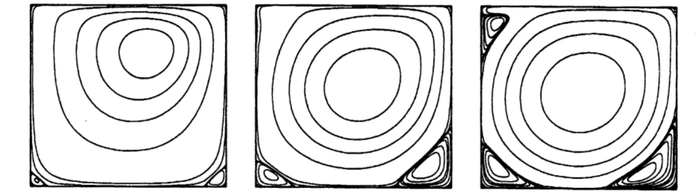
At $t=500$ every solution

was

almost stationary. Figure 4 exhibits the streamlines,

which show the flow patterns well ofthis problem.

Figure 4: Thestreamlinesof$Re=100$ (left), $Re=1$,

000

(center) and$Re=5$,

000

(right)

5 Conclusions

We have presented

a

$8ufficient$ condition for _the _scheme ₍₂₎ _to _be _{stable. In}

_a

_numerical

example

we

have

seen

the condition is reasonable. In another numericalexample

we

have

solved successfully a cavity flow problem with Reynolds numbers up to 5,000.

References

[1] H. Notsu and M. Tabata, A second order characteristic finite element scheme for

the Navier-Stokes equations and

some

numerical simulations, Proceedings of the 20th

Symposium

on

Computational Fluid Dynamics(2006), E5-3 (in Japanese).

[2] H. Rui and M. Tabata, A second order characteristic finite element scheme for

convection-diffusion problems, Numer. Math., $92(2002):161- 177$

.

[3] A. H. Stroud, Approximate calculation of multiple integrals, Prentice-Hall,

1971.

[4] M. Tabata and S. Fujima, Robustness of

a

characteristic flnite element scheme of

second orderin timeincrement, In C. Groth andD. W. Zingg, editors, Computational

Fluid Dynamics 2004, Springer, 177-182,