Measurements of Quantum Interference of Two
Identical Particles with respect to the Event
Plane in Au+Au Collisions at √sNN = 200GeV at
RHIC-PHENIX
著者
新井田 貴文
year
2013
その他のタイトル
RHIC-PHENIX 実験200GeV 金+金衝突における同種2
粒子を用いた量子力学的干渉効果の反応平面依存性
の測定
学位授与大学
筑波大学 (University of Tsukuba)
学位授与年度
2013
報告番号
12102甲第6719号
URL
http://hdl.handle.net/2241/00122770
Measurements of Quantum Interference of Two Identical Particles
with respect to the Event Plane in Au+Au Collisions
at
√
s
NN= 200 GeV at RHIC-PHENIX
Takafumi NIIDA
Measurements of Quantum Interference of Two Identical Particles
with respect to the Event Plane in Au+Au Collisions
at
√
s
NN= 200 GeV at RHIC-PHENIX
Takafumi NIIDA
Doctoral Program in Physics
Submitted to the Graduate School of
Pure and Applied Sciences
in Partial Fulfillment of the Requirements
for the Degree of Doctor of Philosophy in
Science
at the
Abstract
Quark-gluon plasma (QGP) is known as a state of nuclear matter in which the quarks and gluons are deconfined. The Relativistic Heavy Ion Collider (RHIC) at Brookhaven National Laboratory allows us to study the QGP though relativistic nucleus-nucleus collisions. Experimental observables measured at RHIC so far indicate that these nucleus-nucleus collisions lead to the formation of the QGP. The formed QGP expands and cools rapidly, and goes back to a hadronic system as predicted by Quantum Chromodynamics (QCD). The characteristics of the QGP, and the detailed picture of its space-time evolution is emerging by extensive measurements at RHIC. Studies of the final space-time distribution of hadrons and an understanding of its dependence on the initial collision geometry are needed to complete the picture of the space-time evolution of the QGP.
The quantum mechanical interferometry of two identical particles, also known as Hanbury Brown and Twiss (HBT) interferometry, provides us information on the space-time extent of the particle emitting source. Its technique was used to measure the stellar size through the intensity of interference between two photons in the field of astronomy. The same technique have been developed in the field of particle and nuclear physics. In heavy ion collisions, hadron interferometry provides us the space-time extent of hadronic system at the time of last scattering, referred to as kinetic freeze-out. In non-central collisions, it is thought that the collision area is like almond shape at initial state. Then a reaction plane is defined as the plane that the beam axis and the vector connecting the centers of two nuclei make. The larger pressure gradient in the direction of reaction plane due to such a spatial anisotropy leads to the momentum anisotropy called elliptic flow, which is stronger expansion of the source toward the direction of the reaction plane than to the perpendicular direction of that. One may expect the source at kinetic freeze-out change to the shape extended to the direction of the reaction plane. To study the source shape at kinetic freeze-out would be one of the key observables to investigate how and how long the system evolves. The initial density distribution in the collision area has a spatial fluctuation due to the finite number of participating nucleons in addition to the elliptical source shape. Therefore higher order components, such as triangular (3rd-order) flow, or quadrangular (4th-order) flow, etc may be present in both spatial and momentum distribution at kinetic freeze-out. Higher order collective flow have been recently measured, which is thought to primarily come from the initial spatial fluctuations. The initial spatial fluctuations may be preserved until the freeze-out, depending on the strength of the initial fluctuations, flow profile, and expansion time as well as the system temperature, a viscosity, and the source opacity. Therefore the measurement of HBT interferometry with respect to different order event planes, which corresponds to the axes of higher order flows, would be a unique probe of the magnitude of the spatial state fluctuations and the subsequent space-time of a heavy ion collision.
We have performed HBT measurement with respect to 2nd-order event plane in Au+Au colli-sions at√sNN= 200 GeV at the PHENIX experiment. The Gaussian source radii (HBT radii) have
been measured for charged pions and kaons as functions of collision centrality and the transverse mass (mT). Azimuthal angle dependence of the HBT radii have been observed for both species.
Final eccentricities calculated by the pion HBT radii increase with centrality going from central to peripheral collisions and are less than the initial eccentricities in all centralities, which is consistent with the result from STAR experiment. This result indicates that the source strongly expands to the direction of the reaction plane due to the elliptic flow, but is still elliptical and also oriented in the same vertical direction with respect to the reaction plane. On the other hand, the final
2
eccentricity of kaons is larger than that of pions in peripheral events. Because heavier particles get larger momentum by the collective expansion, the emission region of particles will be different even if they have the same momentum. To take into account the effect, the transverse mass (mT)
scaling needs to be considered in the comparison of both species. However the final eccentricity of kaons still shows larger value than that of pions even at the same mT. It have also been found that
azimuthally average HBT radii of kaons are slightly larger than those of pions, and the difference increases with centrality going from peripheral to central collisions. These difference may indicate that pions and kaons have different freeze-out mechanism, and it may be difficult to explain them only by the hadronic rescattering with different cross sections before the freeze-out because positive kaons with less cross section does not show any significant difference compared to negative kaons.
In order to study the details of features at kinetic freeze-out and the difference between particle species, the Blast-wave model fit have been performed for measured HBT radii with the results of the transverse momentum distribution and elliptic flow measured at PHENIX. The Blast-wave model is a kind of hydrodynamics inspired fitting model parameterized by the freeze-out conditions. The obtained parameters corresponding the flow anisotropy and source shape agrees with what we intuitively expect from the results of the elliptic flow and final eccentricity. The extracted freeze-out time (τ ) and the emission duration ∆τ increase with centrality going from peripheral to central collisions (τ =6-8 fm/c, ∆τ =1.5-2.0 fm/c). The extracted freeze-out time shows a similar value obtained by the result from 3D-source imaging analysis with the comparison of a theoretical calculation based on a hydrodynamic expansion including the effect of resonance decays. The result is also closer to a prediction by the hydrodynamic calculation without the hadronic rescattering than the hydrodynamic calculation with the hadronic rescattering. That may suggest that the stage of the hadronic rescattering before the freeze-out is much shorter than expected. The Blast-wave model assumes that the freeze-out of all hadrons takes place at the same time. Therefore the HBT radii of pions and kaons should be explained by the same freeze-out parameters. However the difference between pions and kaons could have not been explained although the transverse momentum distribution and elliptic flow can be explained well for both species. These results may imply that pions and kaon have different freeze-out time or different emission duration during the freeze-out.
We have also performed a first measurement of HBT radii as a function of azimuthal angle with respect to 3rd-order event plane for charged pions. As well as 2nd-order event plane, the angle dependence have been observed although the oscillation amplitudes are smaller than those for 2nd-order. The result in central collisions appears to be qualitatively consistent with a picture that the angle dependence of HBT radii is driven by a finite triangular flow, not a spatial triangular anisotropy, suggested by a recent hydrodynamic model for 3rd-order event plane dependence.
It is known that the dynamical correlation between momentum and spatial distribution affects the HBT radii. For the 3rd-order event plane dependence, both effects of the triangular flow and spatial anisotropy would make the oscillation of HBT radii. In order to disentangle the contribu-tions of spatial and flow anisotropy to azimuthal angle dependence of HBT radii, we have performed a Monte-Carlo simulation including both effects. The simulation results indicate that the initial triangular shape is significantly reduced in central collisions and also implies that initial triangu-larity may be flipped to have an opposite sign at the end of freeze-out by the triangular expansion in peripheral collision. These result would provide important constraints on the dynamics of the QGP, especially for the time scale of the system evolution.
Acknowledgment
I would like to express the deepest appreciation to Prof. Yasuo Miake, who gave me great oppor-tunities for learning not only physics but also a lot of things and had me various experience in my campus life. He also gave me a lot of sound advice on my analysis. My deepest appreciation goes to Prof. ShinIchi Esumi. He gave me insightful comments and useful advice which led to accomplish this thesis. He is always willing to have a discussion about my analysis. I appreciate Prof. Tatsuya Chujo for his useful advice and support which is not only for my research but also life at BNL. I would like to thank Prof. M. Inaba for his professional advice about detectors and electronics. I also would like to express my thanks to Prof. H. Masui for his insightful advice and careful reading of my thesis. I received generous support from Mr. S. Kato, who arranged computer system at Tsukuba.
I would like to express my gratitude to Prof. Akira Ozawa for his careful reading of my thesis. My thesis effectively improved thanks to his useful comments and suggestions.
I want to thank all the members of High Energy Nuclear Physics Group at University of Tsukuba. I express my thanks to Ms. H. Sakai, Mr. Y. Ikeda, Mr. D. Sakata, Mr. M. Sano, Mr. T. Todoroki, Ms. J. Bhom, Mr. S. Mizuno, Mr. H. Nakagomi, Mr. D. Watanabe, Mr. K. Ki-hara, Mr. T. Kobayashi, Mr. K. Oshima, Ms. H. Ozaki, Mr. N. Tanaka, Mr. T. Nonaka, Mr. R. Hosokawa, Mr. W. Sato for their friendship, advice, and encouragement. I want to thank many other colleague including those who already graduated for their advice and discussions. Especially, special thanks to Ms. T. Nakajima for her friendly and humorous encouragement.
I am very grateful to the PHENIX-J group for their financial support. I would like to thank Prof. K. Ozawa for his arrangement for my stay at BNL. I want to thank colleagues in Tokyo University and Hiroshima University, especially thank Mr. M. Nihashi for his many help and friendship. I also would like to express my thanks to Dr. M. Shimomura and Dr. T. Hachiya for their many useful advice, suggestions, and kind help at BNL.
I am deeply grateful to the PHENIX Collaboration. I am grateful to the spokesperson Prof. B. V. Jacak, Prof. J. L. Nagle, and Prof. D. Morrison for their various arrangement and advices. I express my appreciation to Dr. R. Soltz for his many help and useful discussion in writing a paper. I also would like to thank Prof. A. Enokizono for his useful advice on the HBT analysis. I would like to thank the conveners of PLHF (Photons, Light Vector Mesons, Hadrons, and Flow) Physics Working Group, Prof. A. Drees, Prof. K. Shigaki, Dr. T. Sakaguchi, Dr. P. Stankus, and Prof. R. Seto. I express my thanks to Dr. J. S. Haggerty, Dr. M. Chiu. for their many support for the detector works in my stay at BNL. My appreciation also goes to the computing team, especially Dr. C. H. Pinkenburg, Dr. J. Seele. for their support about the data analysis.
I would like to express my thanks to Prof. M. A. Lisa, Prof. S. A. Voloshin, Prof. U. Heinz, and Prof. T. Hirano for their useful advice and valuable discussions on the HBT analysis.
Finally, I would like to thank my family, Toshiko, Keigo, Miwako and Hanae for their continuous support and encouragement. I could never finished this work without their understanding and help.
Contents
1 Introduction 1
1.1 Quantum Chromodynamics . . . 1
1.2 Relativistic Heavy Ion Collisions . . . 4
1.2.1 Space-Time Evolution . . . 4 1.2.2 Collision Geometry . . . 6 1.3 Experimental Observables . . . 8 1.3.1 Energy Density . . . 8 1.3.2 Radial Flow . . . 9 1.3.3 Elliptic Flow . . . 10
1.3.4 Higher-order Harmonic Flow . . . 13
1.3.5 Hanbury-Brown and Twiss Interferometry . . . 14
1.4 Thesis Motivation . . . 19
2 Hanbury-Brown and Twiss Interferometry 20 2.1 History . . . 20
2.2 Theoretical Formalism . . . 20
2.2.1 Quantum Interference of Two Identical Particles . . . 20
2.2.2 Bertsch-Pratt Parameterization . . . 23
2.3 Final State Interaction . . . 24
2.3.1 Coulomb Interaction . . . 24
2.3.2 Other Final State Interaction . . . 25
2.4 Characteristics in Heavy Ion Collisions . . . 26
2.4.1 Dynamical System . . . 26
2.4.2 System Size Dependence . . . 27
2.4.3 Azimuthal Angle Dependence . . . 27
3 Experiment 29 3.1 Relativistic Heavy Ion Collider . . . 29
3.2 PHENIX Experiment . . . 30
3.2.1 Overview of PHENIX . . . 30
3.2.2 Magnet System . . . 32
3.2.3 Global Detectors . . . 32
3.2.4 Central Arm Detectors . . . 37
3.2.5 Summary of PHENIX detectors . . . 46
3.2.6 Data Acquisition System . . . 47 II
CONTENTS III
4 Analysis 49
4.1 Event Selection . . . 49
4.1.1 Centrality Determination . . . 49
4.2 Event Plane Determination . . . 50
4.2.1 Azimuthal Distribution of Emitted Particles . . . 50
4.2.2 Event Plane Determination . . . 52
4.2.3 Event Plane Calibration . . . 52
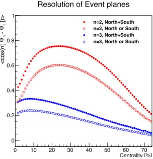
4.2.4 Event Plane Resolution . . . 53
4.3 Track Selection . . . 53 4.3.1 Track Reconstruction . . . 53 4.3.2 Momentum Determination . . . 54 4.3.3 Track Selection . . . 55 4.4 Particle Identification . . . 57 4.5 HBT Analysis Method . . . 58
4.5.1 Construction of Correlation Function . . . 58
4.5.2 Pair Selection . . . 60
4.5.3 Correction of Coulomb Interaction . . . 66
4.5.4 Correction of Momentum Resolution . . . 67
4.5.5 Correction of Event Plane Resolution . . . 72
4.5.6 Fitting Procedure . . . 76
4.6 Initial Spatial Anisotropy . . . 76
4.6.1 Monte-Carlo Glauber Simulation . . . 76
4.6.2 Initial Spatial Anisotropy . . . 77
4.7 Systematic Uncertainties . . . 79
4.7.1 Uncertainties from Track and Pair Selection . . . 79
4.7.2 Uncertainties from Event Plane Determination . . . 80
4.7.3 Uncertainties from Coulomb Correction . . . 80
4.8 Summary of Cut Conditions . . . 86
5 Results 87 5.1 Azimuthally Integrated Measurements . . . 87
5.1.1 Centrality and mT Dependence for Charged Pions . . . 87
5.1.2 Centrality and mT Dependence for Charged Kaons . . . 90
5.2 Azimuthal HBT Measurement with respect to 2nd-order Event Plane . . . 93
5.2.1 Centrality Dependence of HBT Radii for Charged Pions . . . 93
5.2.2 Centrality Dependence of HBT Radii for Charged Kaons . . . 93
5.2.3 kT Dependence of HBT Radii for Charged Pions . . . 94
5.2.4 Comparison with Previous Results . . . 94
5.3 Azimuthal HBT Measurement with respect to 3rd-order Event Plane . . . 100
5.3.1 Centrality Dependence of HBT Radii for Charged Pions . . . 100
5.3.2 kT Dependence of HBT Radii for Charged Pions . . . 100
5.3.3 Comparison with Previous Results . . . 101
6 Discussion 103 6.1 Particle Species Dependence of HBT Radii . . . 103
6.2 Final Source Eccentricity . . . 104
IV CONTENTS
6.2.2 mT Dependence of Final Eccentricity . . . 106
6.3 Interpretation with Blast-wave Model . . . 109
6.3.1 Blast-wave Model . . . 109
6.3.2 Fitting Results . . . 110
6.3.3 Extracted Freeze-out Parameters . . . 113
6.3.4 Systematic Study of the Blast-wave Fit . . . 118
6.4 Final Source Triangularity . . . 120
6.4.1 Centrality and mT Dependence . . . 120
6.4.2 Interpretation with a Monte-Carlo Simulation . . . 124
6.5 Quardrangular Component of Final Source Shape . . . 135
7 Conclusion 137 A Correlation Functions 139 A.1 Correlation Functions of Charged Pions in Azimuthally Integrated Analysis . . . 139
A.2 Correlation Functions of Charged Kaons in Azimuthally Integrated Analysis . . . 139
A.3 Correlation Functions of Charged Pions with respect to 2nd-order Event Plane . . . 148
A.3.1 Centrality Dependence . . . 148
A.3.2 kT Dependence . . . 148
A.4 Correlation Functions of Charged Kaons with respect to 2nd-order Event Plane . . . 148
A.5 Correlation Functions of Charged Pions with respect to 3rd-order Event Plane . . . . 148
A.5.1 Centrality Dependence . . . 148
A.5.2 kT Dependence . . . 148
B Systematic study of HBT radii 161 B.1 kT Dependence of Pion HBT Radii with respect to 2nd-order Event Plane . . . 161
B.2 Kaon HBT Radii with respect to 2nd-order Event Plane . . . 162
B.3 Centrality Dependence of Pion HBT Radii with respect to 3rd-order Event Plane . . 162
B.4 kT Dependence of Pion HBT Radii with respect to 3rd-order Event Plane . . . 162
C Galuber Model 170 C.1 Spatial Eccentricity . . . 170
C.2 Systematic Uncertainties . . . 171
C.3 Data Table of Monte-Carlo Glauber Simulation . . . 173
D Simulation 174 D.1 Generation of Particles . . . 174
D.2 HBT Correlation . . . 174
E Blast wave Model 175 E.1 pT Spectra and Elliptic Flow . . . 175
E.2 HBT Radii . . . 177
List of Figures
1.1 Running coupling constant as a function of momentum transfer Q by the various types of measurements at different scales [2]. The curve is the QCD prediction. . . . 3 1.2 The energy density over T4 as a function of the temperature T scaled by the critical
temperature Tc calculated in Lattice QCD [3]. The arrows indicate the
Stefan-Boltzmann limit of ϵ/T4. . . 4 1.3 Space-time diagram of a relativistic heavy ion collision . . . 7 1.4 Participant-spectator picture in relativistic heavy ion collision. . . 8 1.5 The Bjorken energy density multiplied by the formation time τ for three RHIC
energies [11]. . . 10 1.6 Transverse mass mT distributions for π±, K±, p(¯p) for 3 centrality bins in Au+Au
collisions at √sNN=200 GeV [12]. The solid lines on each spectra represent fitting
results with mT exponential function. . . 11
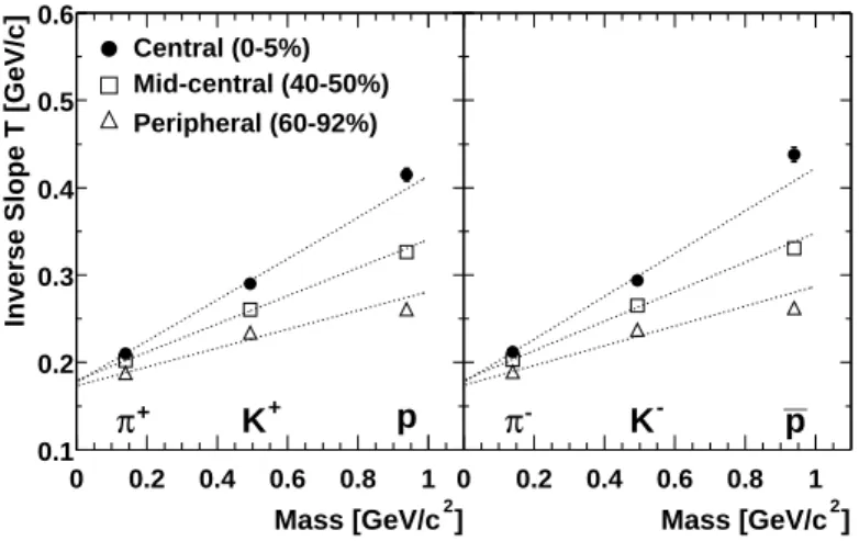
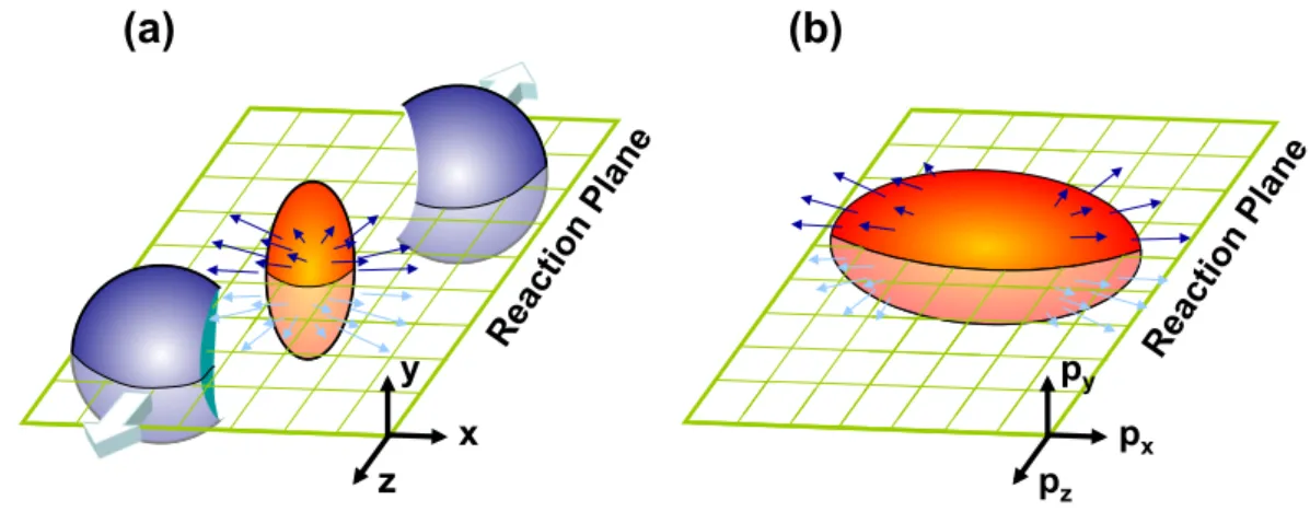
1.7 Mass and centrality dependence of inverse slope parameter T obtained by the fit of exponential function in Fig. 1.6 [12]. The dotted lines are a linear fit of the results with Eq. (1.31). . . 12 1.8 (a)Initial overlap of two nuclei in non central collisions in coordinate space. (b)Collective
flow into the direction of reaction plane in momentum space. . . 13 1.9 (Left)v2 for charged hadrons, π, K, p as a function of pT in Minimum bias events
in Au+Au collisions at √sNN = 200 GeV [15]. (Right)Unscaled and scaled v2 as
functions of KET and KET/nq [17] in 20-60% centrality in Au+Au collisions [17]. . 14
1.10 v2, v3 and v4 as a function of pT for different centrality bins measured with PHENIX. 15
1.11 v2 and v3 as a function of Npart for two pT ranges with the theoretical predictions,
which are hydrodynamic calculations with the Glauber-MC or MC-KLN initial con-dition and different viscosities (4πη/s) and the UrQMD transport model. . . . 16 1.12 (Left)Source radii in Bertcsh Pratt parameterization measured with charged pions as
a function of the mean transverse momentum of pair particles kT [20]. Hydrodynamic
(Hirano [21], Kolb [22], and Zschiesche [23]) and hybrid hydrodynamic/cascade (Soff) model calculation are compared. (Right)Source radii calculated by the improved hy-drodynamic model with several conditions (symbols with lines), where experimental data from STAR (red star) are compared [25]. . . 17 1.13 Azimuthal angle dependence of HBT radii calculated by the hydrodynamic model [26],
assuming the impact parameter b=7 fm and Au+Au collisions at √sNN=130 GeV. . 18
1.14 A sketch of the evolution of the system shape in coordinate space after the collision. 18 2.1 Conceptual diagram of quantum interference between two identical particles. . . 21 2.2 Schematic figure of Bertsch-Pratt parameterization. The relative momentum of pair
particles is decomposed into a longitudinal, sideward and outward direction. . . 23 V
VI LIST OF FIGURES
2.3 A sketch of the emission region for a static source (a) and a dynamical expanding source (b). In the expanding source, it is assumed that the transverse velocity βT of
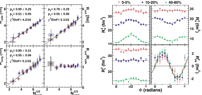
particles is proportional to the distance from the center of the source to their particle positions. . . 26 2.4 (Left)The HBT radii and the ratio of Rs and Ro for positive (blue square) and
negative (red triangle) pion pairs as a function of Npart1/3 in Au+Au collisions at √
sNN= 200 GeV, measured at the PHENIX experiment [36]. (Right)Squared HBT
radii with respect to 2nd-order event plane for three centrality bins measured at the STAR experiment [64]. . . 28 3.1 Aerial photograph of the RHIC facility . . . 29 3.2 The layout of PHENIX detectors in 2007 RHIC-run configuration. Top figure is the
central arm detectors viewed from the beam axis. Bottom figure is side view of the global detectors and muon arm detectors. . . 31 3.3 Line drawings of the PHENIX magnets, shown in perspective and cut away to show
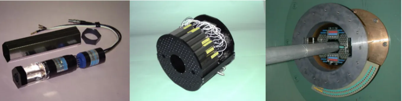
the interior structures. Arrows indicate the line of the colliding beams in RHIC. . . 32 3.4 (Left)An element of the BBC composed of a mesh-dynode photomultiplier with a
quartz radiator. (Middle)A BBC composed of 64 elements. (Right)The BBC in-stalled around the beam pipe behind the Central Magnet. . . 33 3.5 (A)Plain view along the beam axis indicating the location of the BBC, the DX dipole
magnet and the ZDC. (B)Cross-section view of Figure (A) along the A-A line. . . . 34 3.6 (Left)Schematic of a ZDC module. (Right)A photo of a ZDC module. . . 35 3.7 Schematic view of the Reaction Plane Detector . . . 36 3.8 Photo of the RXNP installed on the nosecone of the PHENIX central magnet in
north side, where four quadrants surround the beam pipe. . . 36 3.9 The frame of the Drift Chambers . . . 37 3.10 (Left)The layout of wire position within one DC sector and inside the anode plane.
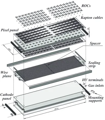
(Right)Top view of the stereo wire orientation. . . 38 3.11 The principle of the pad geometry . . . 39 3.12 Exploded view of a PC1 chamber . . . 40 3.13 (Left) Photo of the TOF.E detector mounted on the PHENIX east arm. (Right)
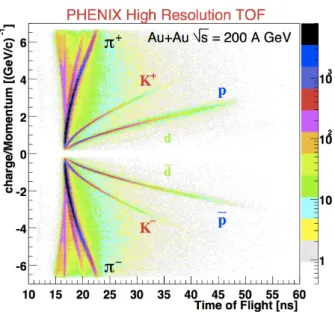
Schematic diagram of the components of a single TOF.E panel. . . 41 3.14 Contour plot of the time of flight versus reciprocal momentum in minimum bias
Au+Au collisions. . . 41 3.15 Cross sectional view of the TOF.W MRPC. . . 42 3.16 (Left)Side view of a MRPC chamber (Right)A panel of TOF.W consisting of 32
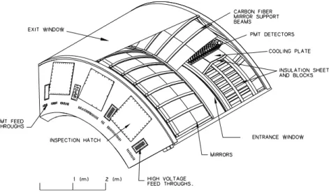
MRPC chambers. . . 43 3.17 A cutaway view of a RICH detector showing the spherical mirrors and PMTs inside. 44 3.18 Interior view of a Pb-scintillator calorimeter module showing a stack of scintillator
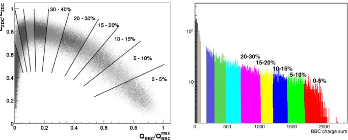
and lead plates, wavelength hitting fiber readout and leaky fiber inserted in the central hole. . . 45 3.19 Schematic diagram of the PHENIX DAQ system. . . 47 4.1 (Left) Correlation between the total energy measured in the ZDC and the charge
sum deposited in the BBC. (Right) Distribution of the charge sum deposited in the BBC. . . 50
LIST OF FIGURES VII
4.2 Event plane resolution as a function of centrality in Au+Au collisions at√sNN= 200
GeV. The resolution for the North or South RXNP and the combined subdetectors are shown. . . 54 4.3 The schematic view of a reconstructed track by the DC in x− y plane (Left) and
r− z plane (Right). . . 55 4.4 (Left)The DC hits in x− y plane. (Right)The hit distribution in Hough space [49]. . 56 4.5 Squared mass distribution in the pT region of 0.9 ≤ pT < 1.0 GeV/c. Solid lines
show triple Gaussian fit functions and dashed lines show each component of them. . 57 4.6 Mean (left) and width (right) of squared mass distribution as a function of
momen-tum for π/K/p. Filled (open) symbols represent positive (negative) particles. . . . . 58 4.7 Momentum multiplied by a sign of charged track vs mass square for Particle
Identi-fication by EMCal. . . 59 4.8 Relative momentum distributions for real and mixed pairs (Upper panel) and a
correlation function obtained by the ratio of real and mixed pair q-distributions in upper panel (Lower Panel). . . 60 4.9 Ratio of real and mixed pion pairs as functions of the relative difference in dz-dϕ
plane at the DC in 0-10% centrality, where mixed pairs is normalized so that the total number of pair over 50< dz <100 cm and 0.1< dϕ <0.2 rad. should be equal between real and mixed pairs. . . 61 4.10 Ratio of real and mixed pairs as functions of the relative difference at the EMC in
0-10% centrality, where mixed pairs are normalized, so that the total number of pair over 50< dr <100 cm should be equal between real and mixed pairs. . . . 62 4.11 Ratio of real and mixed pion pairs as a function of the relative angular difference dϕ
every dz with 1 cm step. This plot is a slice of Fig. 4.9. . . . 63 4.12 Ratio of real and mixed kaon pairs as functions of the relative difference in dz-dϕ
plane at the DC in 0-60% centrality, where mixed pairs is normalized, so that the total number of pair over 50< dz <100 cm and 0.1< dϕ <0.2 rad. should be equal between real and mixed pairs. . . 64 4.13 Real pairs, mixed pairs, and the ratio of real and mixed pairs for charged kaons as
functions of dz and dϕ at the EMC in 0-60%. . . . 64 4.14 Ratio of real and mixed kaon pairs as a function of the relative angular difference
dϕdc every dzdc with 1 cm step. . . 65
4.15 Measured 1-dimensional correlation function (filled circles) of charged pion pairs as a function qinv with the fit function (solid line) of Eq.(4.36). Coulomb correction
factor Fcoul(qinv) calculated by the Coulomb wave function is shown as open symbols. 67
4.16 Difference of pT, ϕ, θ between the generated particles and reconstructed tracks in
the simulation as a function of momentums. . . 68 4.17 Momentum resolution for positive pions in the different magnetic fields. The
stan-dard deviations and means of ∆pT/pT, ∆ϕ, ∆θ distribution obtained by the Gaussian
fit are plotted as a function momentum. . . 69 4.18 Momentum resolution for negative pions in the different magnetic fields. The
stan-dard deviations and means of ∆pT/pT, ∆ϕ, ∆θ distribution obtained by the Gaussian
fit are plotted as a function momentum. . . 69 4.19 Momentum resolution for charged pions with polynomial fit. The standard deviations
of ∆pT/pT, ∆ϕ, ∆θ distribution obtained by the Gaussian fit are plotted as a function
VIII LIST OF FIGURES
4.20 Momentum resolution for positive kaons in +− magnetic field. The standard devia-tions of ∆pT/pT, ∆ϕ, ∆θ distribution obtained by the Gaussian fit are plotted as a
function momentum, where the result of pions are compared. . . 70 4.21 Extracted 3D-HBT radii with and without momentum resolution correction . . . 71 4.22 Illustration of the smearing effect for the measured source size by the finite event
plane resolution. . . 72 4.23 Corrected and uncorrected 3D HBT radii as a function of azimuthal pair angle
relative to Ψ2 (∆ϕ) in HBT simulation with a bad event plane resolution. . . . 73
4.24 Uncorrected 3D HBT radii as a function of azimuthal pair angle relative to Ψ3 (∆ϕ)
for different event plane resolution in HBT simulation. . . 74 4.25 Corrected 3D HBT radii as a function of azimuthal pair angle relative to Ψ3 (∆ϕ)
for different event plane resolution in HBT simulation. . . 75 4.26 Corrected and uncorrected 3D HBT radii of charged pions as a function of azimuthal
pair angle relative to Ψ2 (∆ϕ) in Au+Au collisions at √sNN = 200 GeV. . . 75
4.27 (Left) The number of participants distribution and that for each divided centrality classes. (Right) Impact parameter distribution and that for each divided centrality classes. . . 77 4.28 (Left) Npartas a function of centrality in Glauber simulation. PHENIX official values
in Run7 are compared. (Right) Eccentricity as a function of centrality. Standard and participant eccentricity in PHENIX and my simulation are shown. . . 78 4.29 Initial higher order anisotropy as a function of centrality. ε4 is calculated for both
Ψ2 and Ψ4. Systematic errors are shown together. . . 79
4.30 Squared HBT radii of charged pions with different conditions of track matching cut. 81 4.31 Squared HBT radii of charged pions with different conditions of PID cut and pair
selection cut. . . 81 4.32 Squared HBT radii of charged pions measured with different event planes. . . 82 4.33 Squared HBT radii of charged pions with different input source size for Coulomb
strength. . . 82 5.1 3D HBT parameters of charged pions as a function of mT for four centrality bins,
where only the statistical errors are shown. . . 87 5.2 3D HBT parameters of charged pions as a function of mT in 0-30% with the
com-parison of the PHENIX result [36]. . . 88 5.3 Comparison of the mT dependence of 3D HBT parameters of charged pions with the
STAR result [62]. . . 89 5.4 3D HBT parameters of positive and negative kaon pairs as a function of mT for four
centrality bins. . . 90 5.5 3D HBT parameters of charged kaons as a function of mT for four centrality bins,
where positive and negative kaon pairs are combined. . . 91 5.6 3D HBT parameters of positive and negative kaon pairs as a function of mT for two
centrality bins. . . 92 5.7 3D HBT parameters of charged kaons as a function of mT for two centrality bins,
LIST OF FIGURES IX
5.8 Projected 3D correlation functions of charged pion pairs in 0.2 < kT < 2.0 GeV/c at
four centrality bins without the correction of the event plane resolution. Correlation functions at ∆ϕ = 0 (red symbol) and ∆ϕ = π/2 (blue symbol) are shown. Correla-tion funcCorrela-tions are projected along each q direcCorrela-tions with qother< 50 [MeV/c]. Solid
lines show the fit functions by Eq. (4.36), which is also projected in the same way. . 95 5.9 Extracted HBT parameters of charged pions in 0.2 < kT < 2.0 GeV/c as a function
of azimuthal pair angle with respect to 2nd-order event plane for four centrality bins with systematic uncertainties (shaded bands). The data point at ∆Φ = π is the same value as the data at ∆Φ = 0. . . 96 5.10 Extracted HBT parameters of charged pions in 0.2 < kT < 2.0 GeV/c as a function
of azimuthal pair angle with respect to 2nd-order event plane for four centrality bins. The data point at ∆Φ = π is same value at ∆Φ = 0. Solid lines depict fit functions by Eq. (5.1). . . 96 5.11 Projected 3D correlation functions of charged kaon pairs in 0.3 < kT < 2.0 GeV/c
at 0-20% and 20-60% centrality without the correction of the event plane resolution. Correlation functions at ∆ϕ = 0 (red symbol) and ∆ϕ = π/2 (blue symbol) are shown. Correlation functions are projected along each q directions with qother < 50
[MeV/c]. Solid lines show the fit functions. . . 97 5.12 Extracted HBT parameters of charged kaons in 0.3 < kT < 2.0 GeV/c as a function
of azimuthal pair angle with respect to 2nd-order event plane in two centrality bins, where shaded bands show the systematic uncertainties. The data point at ∆Φ = π is the same value at ∆Φ = 0. Solid lines depict the fit function by Eq. (5.1) . . . 97 5.13 Extracted HBT parameters of charged pions as a function of azimuthal pair angle
with respect to 2nd-order event plane for six kT bins. Solid band lines represent
systematic uncertainties. The data point at ∆Φ = π is the same value at ∆Φ = 0. . 98 5.14 Extracted HBT parameters of charged pions as a function of azimuthal pair angle
with respect to 2nd-order event plane for six kT bins with fit functions by Eq. (5.1).
The data point at ∆Φ = π is the same value at ∆Φ = 0. . . . 98 5.15 3D HBT parameters of charged pions and kaons as a function of Npart1/3. Averages of
HBT parameters measured in different azimuthal angle with respect to Ψ2 are
com-pared with the results of azimuthally integrated analysis published in the PHENIX experiment [36, 66], where color bands represent the systematic uncertainties. . . 99 5.16 3D HBT parameters as a function of average mT. Averages of HBT parameters
measured in different azimuthal angle with respect to Ψ2 are compared with the
results of azimuthally integrated analysis published in the STAR experiment [62], where color bands represent the systematic uncertainties. . . 99 5.17 Extracted HBT parameters of charged pions in 0.2 < kT < 2.0 GeV/c as a function
of azimuthal pair angle with respect to 3rd-order event plane for four centrality classes, where shaded bands show the systematic uncertainties. The data point at ϕ− Φ = 2π/3 is same value at ϕ − Φ = 0. The solid lines depict the fit functions by Eq. (5.1). . . 100 5.18 3D HBT radii of charged pions as a function of azimuthal pair angle with respect
to 3rd-order event plane for five k
T bins and two centrality bins, 0-20% (Left) and
20-60% (Right). The data point at ϕ− Φ = 2π/3 is the same value at ϕ − Φ = 0. Band consisting of two thin lines represent the systematic uncertainties and normal solid lines depict the fit functions by Eq.(5.1). The R2
os is plotted with respect to
X LIST OF FIGURES
5.19 3D HBT radii of charged pions as a function of Npart1/3. Averages of azimuthally Ψ3
dependent radii are compared with the results of azimuthally integrated analysis published in PHENIX [36]. Color bands show the systematic uncertainties. . . 102 6.1 Comparison of mT dependence of HBT radii between charged pions and kaons for
four centrality bins. . . 104 6.2 Comparison of Ro/Rs between charged pions and kaons. . . 105
6.3 Initial eccentricity vs final eccentricity for charged pions and kaons. The kT ranges
are 0.2 < kT < 2.0 GeV/c for pions and 0.3 < kT < 2.0 GeV/c for kaons. The initial
eccentricity is calculated by a Monte-Carlo Glauber simulation, where color bands shows the systematic uncertainties. A band consisting of two solid lines represents the 30% systematic uncertainties derived from the definition of the final eccentricity [67]. Result for pions measured by STAR [64] experiment is also shown. Dashed line shows εinitial= εf inal. . . 106
6.4 Relative amplitudes of azimuthal HBT radii for charged pions and kaons with re-spect to 2nd-order event plane, where color bands shows the systematic uncertainties. Dashed lines show the line of x-axis=y-axis. . . 107 6.5 Relative amplitude of azimuthal HBT radii for charged pions and kaons with respect
to 2nd-order event plane as a function of mT in two centrality bins in Au+Au 200
GeV collisions, where color bands shows the systematic uncertainties. The relative ratio of Rs shown in the left top panel corresponds to the εf inal. . . 108
6.6 Azimuthal oscillations and relative amplitudes of the HBT radii calculated by an ideal hydrodynamic model [26] with b=7 fm Au+Au collisions at √sNN=130 GeV,
for 4 kT values. Data points are read from the figures in [26]. . . 108
6.7 (Left) Blast-wave fit for pT spectra of π, K, p in two centrality bins [12]. Solid black
lines show the fit functions with the best fit parameters and actual fit range, and color lines shows the extended fit functions. (Right) χ2 contour plot as functions of Tf and ρ0. Solid lines show 1σ, 2σ, and 3σ contour lines and red points show the
best fit parameters. . . 111 6.8 Blast-wave fit for v2 of π++ π−, K++ K−, p + ¯p [70]. Solid black lines show the
fit functions with the best fit parameters and actual fit range, and color lines shows the extended fit functions. . . 111 6.9 Blast-wave fit for pion HBT radii for 6 kT bins and two centralities, 0-20%(Left) and
20-60%(Right). Red solid lines show the Blast-wave fit functions. . . 112 6.10 mT dependence of the mean 3D HBT radii for charged pions with the Blast-wave fit
lines, where the fit is applied for v2 and azimuthal angle dependence of HBT radii
using Tf and ρ0 fixed by pT spectra. . . 112
6.11 (Left) χ2 contour plot as functions of ρ2 and Ry/Rx. (Right) χ2 contour plot as
functions of τ and ∆τ . Red points show the best fit parameters. . . . 113 6.12 Extracted freeze-out parameters as a function of Npart. Color boxes show the
sys-tematic uncertainties. . . 114 6.13 The spatial weighting function Ω for as = 0 (box profile) and as=0.1. . . 115
6.14 Extracted freeze-out parameters as a function of Npart. . . 115
6.15 Average HBT radii of pions and kaons calculated by the Blast-wave model as a function of mT, where the wave model parameters are obtained by the
LIST OF FIGURES XI
6.16 Comparison of the data and Blast-wave model calculations using fit results for the mT dependence of relative amplitudes in two centrality regions. Blast-wave model
calculations of kaons using the extracted parameters by spectra, v2 and pion HBT. . 117
6.17 Extracted freeze-out parameters as a function of Npart for various combinations of
observables used in the Blast-wave fit. The Tf and ρ0 are obtained by pT spectra
fit, and other parameters are obtained by a simultaneous fit for v2 and HBT radii. . 118
6.18 The azimuthal angle dependence of Rs2 and R2o for charged pions with respect to 2nd and 3rd-order event plane in Au+Au collisions at √s
NN=200 GeV. Filled symbols
show the extracted HBT radii and open symbols are the same data symmetrized from −π to π rad as filled symbols. Color bands consisting of two thin lines represent the systematic uncertainties. . . 121 6.19 Relative amplitudes of squared HBT radii with respect to 2nd and 3rd-order event
planes as a function of initial εn, where the initial εn is calculated by a Monte-Carlo
Glauber model. Color boxes represent the systematic uncertainties. . . 122 6.20 Relative amplitudes of squared HBT radii with respect to 3rd-order event plane as
a function of mT for two different centrality bins, where color boxes represent the
systematic uncertainties. . . 122 6.21 R2s and R2o as a function of emission angle Φ with respect to Ψ3 (Left) and kT
dependence of the 3rd-order oscillation amplitudes of Rs2 and R2o (Right ) for the “geometry-dominated-source” (thin red lines or (a)) and “flow-dominated-source” (thick blue lines or (b)) calculated by a hydrodynamic model with a simple Gaussian source. These figures are taken from [71]. . . 123 6.22 mT dependence of the 3rd-order oscillation amplitudes of R2s and R2o with the
com-parison of a hydrodynamic model with a simple Gaussian source [71]. . . 123 6.23 Scatter plots of generated particles in x− y plane for elliptical (n=2) and triangular
(n=3) source, where R0 = 5 fm, a = 0.54. . . 124
6.24 Transverse velocity with β0= 0.8 and βn= 0. . . 125
6.25 Boost angle of simulated particles ((Left)elliptical source (Right)triangular source). Dots represent particle elements consisting of the source, black lines show the radial direction from the center of the source, and magenta lines show the perpendicular direction to the surface of the source. . . 126 6.26 Inverse slope parameter as a function of particle mass. Simulation and experimental
results are compared. . . 127 6.27 Tuned R2
s and Ro2 as a function of azimuthal angle with respect to 2nd-order event
plane, where the parameter R0 and ∆τ are tuned. . . . 128
6.28 kT dependence of the mean Rs and Ro with the parameters of 0-10% shown in
Table 6.4, where resuls using three different ∆τ are shown. Experimental results are also shown. . . 128 6.29 Transverse mass (mT) dependence of the relative Rsand Rofor 3rd-order event plane
in two centrality bins. Open symbols with dotted and dashed lines are calculated by MC-simulation. . . 129 6.30 Relative amplitudes of R2s and R2o as a function of e2 for various β2 for the radial
boost, where the parameters for 0-10% shown in Table 6.4are used. . . 130 6.31 Relative amplitudes of R2s and R2o as a function of e3 for various β3 for the radial
boost, where the parameters for 0-10% shown in Table 6.4are used. . . 130 6.32 Relative amplitudes of R2
s and R2o as a function of e2 for various β2 for the
XII LIST OF FIGURES
6.33 Relative amplitudes of Rs2 and R2o as a function of e3 for various β3 for the
perpen-dicular boost, where the parameters for 0-10% shown in Table 6.4are used. . . 131 6.34 v2as a function of pT for different e2and β2for the radial boost, where the parameters
for 0-10% shown in Table 6.4are used. . . 131 6.35 v3as a function of pT for different e3and β3for the radial boost, where the parameters
for 0-10% shown in Table 6.4are used. . . 131 6.36 v2 as a function of pT for different e2 and β2 for the perpendicular boost, where the
parameters for 0-10% shown in Table 6.4are used. . . 132 6.37 v3 as a function of pT for different e3 and β3 for the perpendicular boost, where the
parameters for 0-10% shown in Table 6.4are used. . . 132 6.38 Contour map of χ2 between data and simulation for 2nd- and 3rd-order, where the
χ2 is calculated from the relative amplitudes of Ro and Rs, and vn. Shaded areas
represent the regions within 2-σ contour for 2nd-order HBT and 1-σ contour for 3rd-order HBT, and 4-σ contour for v
n. . . 133
6.39 Contour map of χ2 between data and simulation for 2nd- and 3rd-order, where the χ2 is calculated from the relative amplitudes of Ro and Rs, and vn. Shaded areas
represent the regions within 2-σ contour for 2nd-order HBT and 1-σ contour for 3rd-order HBT, and 4-σ contour for vn. . . 134
6.40 Fourier decompositions of R2s and Ro2 relative to 2nd-order event plane for charged pions. . . 135 6.41 Relative 4th-order Fourier coefficients of R2s and R2o as a function of initial ε4(Ψ2)
calculated by a Monte-Carlo Glauber simulation. . . 136 A.1 Correlation functions of charged pion pairs in 0-10% centrality, where solid lines
show the fit functions. Filled symbols show positive pion pairs and open symbols show negative pion pairs. . . 140 A.2 Correlation functions of charged pion pairs in 10-20% centrality, where solid lines
show the fit functions. Filled symbols show positive pion pairs and open symbols show negative pion pairs. . . 141 A.3 Correlation functions of charged pion pairs in 20-40% centrality, where solid lines
show the fit functions. Filled symbols show positive pion pairs and open symbols show negative pion pairs. . . 142 A.4 Correlation functions of charged pion pairs in 40-70% centrality, where solid lines
show the fit functions. Filled symbols show positive pion pairs and open symbols show negative pion pairs. . . 143 A.5 Correlation functions of charge combined kaon pairs in 0-10% centrality, where solid
lines show the fit functions. . . 144 A.6 Correlation functions of charge combined kaon pairs in 10-20% centrality, where solid
lines show the fit functions. . . 144 A.7 Correlation functions of charge combined kaon pairs in 20-40% centrality, where solid
lines show the fit functions. . . 145 A.8 Correlation functions of charge combined kaon pairs in 40-70% centrality, where solid
lines show the fit functions. . . 145 A.9 Correlation functions of charged kaon pairs in 0-10% centrality, where solid lines
show the fit functions. . . 146 A.10 Correlation functions of charged kaon pairs in 10-20% centrality, where solid lines
LIST OF FIGURES XIII
A.11 Correlation functions of charged kaon pairs in 20-40% centrality, where solid lines show the fit functions. . . 147 A.12 Correlation functions of charged kaon pairs in 40-70% centrality, where solid lines
show the fit functions. . . 147 A.13 Projected 3D correlation functions of charged pion pairs measured with respect to
2nd-order event plane for 0.2 < k
T < 2.0 GeV/c with the correction of the event
plane resolution. Correlation functions at ∆ϕ = 0 (red symbol) and ∆ϕ = π/2 (blue symbol) are shown. Correlation functions are projected along each q directions with qother < 50 [MeV/c]. Solid lines show the fit functions. . . 149
A.14 Projected 3D correlation functions of charged pion pairs measured with respect to 2nd-order event plane for 0.2 < k
T < 2.0 GeV/c at five kT bins in 0-20% centrality
bin without the correction of the event plane resolution. Correlation functions at ∆ϕ = 0 (red symbol) and ∆ϕ = π/2 (blue symbol) are shown. Correlation functions are projected along each q directions with qother< 50 [MeV/c]. Solid lines show the
fit functions. . . 150 A.15 Projected 3D correlation functions of charged pion pairs measured with respect to
2nd-order event plane for 0.2 < kT < 2.0 GeV/c at five kT bins in 20-60% centrality
bin without the correction of the event plane resolution. Correlation functions at ∆ϕ = 0 (red symbol) and ∆ϕ = π/2 (blue symbol) are shown. Correlation functions are projected along each q directions with qother< 50 [MeV/c]. Solid lines show the
fit functions. . . 151 A.16 Projected 3D correlation functions of charged pion pairs measured with respect to
2nd-order event plane for 0.2 < kT < 2.0 GeV/c at five kT bins in 0-20% centrality bin
with the correction of the event plane resolution. Correlation functions at ∆ϕ = 0 (red symbol) and ∆ϕ = π/2 (blue symbol) are shown. Correlation functions are projected along each q directions with qother< 50 [MeV/c]. Solid lines show the fit
functions. . . 152 A.17 Projected 3D correlation functions of charged pion pairs measured with respect to
2nd-order event plane for 0.2 < k
T < 2.0 GeV/c at five kT bins in 20-60% centrality
bin with the correction of the event plane resolution. Correlation functions at ∆ϕ = 0 (red symbol) and ∆ϕ = π/2 (blue symbol) are shown. Correlation functions are projected along each q directions with qother< 50 [MeV/c]. Solid lines show the fit
functions. . . 153 A.18 Projected 3D correlation functions of charged kaon pairs measured with respect
to 2nd-order event plane for 0.3 < kT < 2.0 GeV/c at 0-20% centrality with the
correction of the event plane resolution. Correlation functions at ∆ϕ = 0 (red symbol) and ∆ϕ = π/2 (blue symbol) are shown. Correlation functions are projected along each q directions with qother< 50 [MeV/c]. Solid lines show the fit functions. . 154
A.19 Projected 3D correlation functions of charged pion pairs measured with respect to 3rd-order event plane for 0.2 < kT < 2.0 GeV/c at four centrality bins without
the correction of the event plane resolution. Correlation functions at ∆ϕ = 0 (red symbol) and ∆ϕ = π/3 (blue symbol) are shown. Correlation functions are projected along each q directions with qother< 50 [MeV/c]. Solid lines show the fit functions. . 155
XIV LIST OF FIGURES
A.20 Projected 3D correlation functions of charged pion pairs measured with respect to 3rd-order event plane for 0.2 < kT < 2.0 GeV/c at four centrality bins with the
correction of the event plane resolution. Correlation functions at ∆ϕ = 0 (red symbol) and ∆ϕ = π/3 (blue symbol) are shown. Correlation functions are projected along each q directions with qother< 50 [MeV/c]. Solid lines show the fit functions. . 156
A.21 Projected 3D correlation functions of charged pion pairs measured with respect to 3rd-order event plane for 0.2 < kT < 2.0 GeV/c at five kT bins without the correction
of the event plane resolution. Correlation functions at ∆ϕ = 0 (red symbol) and ∆ϕ = π/3 (blue symbol) are shown. Correlation functions are projected along each q directions with qother< 50 [MeV/c]. Solid lines show the fit functions. . . 157
A.22 Projected 3D correlation functions of charged pion pairs measured with respect to 3rd-order event plane for 0.2 < kT < 2.0 GeV/c at five kT bins without the correction
of the event plane resolution. Correlation functions at ∆ϕ = 0 (red symbol) and ∆ϕ = π/3 (blue symbol) are shown. Correlation functions are projected along each q directions with qother< 50 [MeV/c]. Solid lines show the fit functions. . . 158
A.23 Projected 3D correlation functions of charged pion pairs measured with respect to 3rd-order event plane for 0.2 < kT < 2.0 GeV/c at five kT bins with the correction
of the event plane resolution. Correlation functions at ∆ϕ = 0 (red symbol) and ∆ϕ = π/3 (blue symbol) are shown. Correlation functions are projected along each q directions with qother< 50 [MeV/c]. Solid lines show the fit functions. . . 159
A.24 Projected 3D correlation functions of charged pion pairs measured with respect to 3rd-order event plane for 0.2 < kT < 2.0 GeV/c at five kT bins with the correction
of the event plane resolution. Correlation functions at ∆ϕ = 0 (red symbol) and ∆ϕ = π/3 (blue symbol) are shown. Correlation functions are projected along each q directions with qother< 50 [MeV/c]. Solid lines show the fit functions. . . 160
B.1 HBT parameters of charged pions in 0.2 < kT < 2.0 GeV/c as a function of azimuthal
pair angle with respect to 2nd-order event plane in six kT and two centrality bins
with different matching cuts. . . 161 B.2 HBT parameters of charged pions in 0.2 < kT < 2.0 GeV/c as a function of azimuthal
pair angle with respect to 2nd-order event plane in six kT and two centrality bins
with different PID cut. . . 162 B.3 HBT parameters of charged pions in 0.2 < kT < 2.0 GeV/c as a function of azimuthal
pair angle with respect to 2nd-order event plane in four kT and two centrality bins
with different event planes. . . 163 B.4 HBT parameters of charged pions in 0.2 < kT < 2.0 GeV/c as a function of azimuthal
pair angle with respect to 2nd-order event plane in four kT and two centrality bins
with different input source size for the calculation of the Coulomb interaction. . . . 163 B.5 HBT parameters of charged kaons in 0.3 < kT < 2.0 GeV/c as a function of azimuthal
pair angle with respect to 2nd-order event plane in two centrality bins with different matching cut. . . 164 B.6 HBT parameters of charged kaons in 0.3 < kT < 2.0 GeV/c as a function of azimuthal
pair angle with respect to 2nd-order event plane in two centrality bins with different PID cut. . . 164 B.7 HBT parameters of charged kaons in 0.3 < kT < 2.0 GeV/c as a function of azimuthal
pair angle with respect to 2nd-order event plane in two centrality bins with different
LIST OF FIGURES XV
B.8 HBT parameters of charged kaons in 0.3 < kT < 2.0 GeV/c as a function of azimuthal
pair angle with respect to 2nd-order event plane in two centrality bins with different input source size for the calculation of the Coulomb interaction. . . 165 B.9 HBT parameters of charged pions in 0.2 < kT < 2.0 GeV/c as a function of azimuthal
pair angle with respect to 3rd-order event plane in four centrality bins with different matching cuts. . . 165 B.10 HBT parameters of charged pions in 0.2 < kT < 2.0 GeV/c as a function of azimuthal
pair angle with respect to 3rd-order event plane in four centrality bins with different PID cut. . . 166 B.11 HBT parameters of charged pions in 0.2 < kT < 2.0 GeV/c as a function of azimuthal
pair angle with respect to 3rd-order event plane in four centrality bins with different event planes. . . 166 B.12 HBT parameters of charged pions in 0.2 < kT < 2.0 GeV/c as a function of azimuthal
pair angle with respect to 3rd-order event plane in four centrality bins with different input source size for the calculation of the Coulomb interaction. . . 167 B.13 HBT parameters of charged pions in 0.2 < kT < 2.0 GeV/c as a function of azimuthal
pair angle with respect to 3rd-order event plane in five kT and two centrality bins
with different matching cuts. . . 167 B.14 HBT parameters of charged pions in 0.2 < kT < 2.0 GeV/c as a function of azimuthal
pair angle with respect to 3rd-order event plane in five kT and two centrality bins
with different PID cut. . . 168 B.15 HBT parameters of charged pions in 0.2 < kT < 2.0 GeV/c as a function of azimuthal
pair angle with respect to 3rd-order event plane in five kT and two centrality bins
with different event planes. . . 168 B.16 HBT parameters of charged pions in 0.2 < kT < 2.0 GeV/c as a function of azimuthal
pair angle with respect to 3rd-order event plane in five kT and two centrality bins
with different input source size for the calculation of the Coulomb interaction. . . . 169 C.1 Npart(left) and εstdcalculated with different input parameters of Glauber simulation
are plotted as a function of centrality. PHENIX official values in Run7 are compared. 172 C.2 εpart (left) and ε3 calculated with different input parameters of Glauber simulation
are plotted as a function of centrality. PHENIX official values in Run7 are compared for εpart. . . 172
C.3 ε4 calculated with different input parameters of Glauber simulation are plotted as a
function of centrality, where ε4 is calculated for both Ψ2 and Ψ4. . . 172
E.1 Blast-wave fit of HBT radii in the fit B. . . 177 E.2 Blast-wave fit of HBT radii in the fit C, 0-20%(Left) and 20-60%(Right). . . 178 E.3 Blast-wave fit of HBT radii in the fit D. . . 178 E.4 Blast-wave fit of v2 in the fit B. . . 179
E.5 Blast-wave fit of v2 in the fit C. . . 179
List of Tables
1.1 Summary of heavy ion collider facilities with the ion beams and the center of mass energy. . . 5 3.1 Summary of PHENIX detector subsystems . . . 46 4.1 Summary of systematic errors for squared HBT radii of pions for four centralities.
The errors at ∆ϕ=0, π/4, π/2, 3π/4 are shown. . . . 83 4.2 Summary of systematic errors for squared HBT radii of pions for four centralities.
The errors at ∆ϕ=0, π/4, π/2, 3π/4 are shown. . . . 84 4.3 Summary of systematic errors for squared HBT radii of kaons for four centralities.
The errors at ∆ϕ=0, π/4, π/2, 3π/4 are shown. . . . 85 4.4 Summary of cut conditions . . . 86 6.1 Extracted parameters by the Blast-wave fit. The Tf and ρ0 are obtained by pT
spectra fit for π, K, p, and other parameters are obtained by a simultaneous fit for v2 of π, K, p and pion HBT radii. The value inside () represents the systematic error.113
6.2 Fit range in the Blast-wave fit . . . 115 6.3 Summary of extracted parameters of the Blast-wave model for different fit conditions.
The Tf and ρ0are obtained by pT spectra fit, and other parameters are obtained by a
simultaneous fit for v2 and HBT radii. The value inside () represents the systematic
error. . . 119 6.4 Summary of simulation parameters . . . 126 6.5 Search conditions of en and βn . . . 127
C.1 The number of participants and initial eccentricity with respect to higher-order par-ticipant plane angle calculated by Monte-Carlo Glauber simulation . . . 173
Chapter 1
Introduction
It is well known that the matter existing around us consists of various kinds of atoms and molecules. The atom have a nuclei in the center and electrons exist around the nuclei like a cloud. Furthermore the nuclei is composed of protons and neutrons called the nucleon. Protons and neutrons are composed of three quarks. Thus the matter is composed of smaller particles hierarchically, which is called hierarchical structure of the matter.
At present, the most fundamental particles composing the matter are believed to be quarks, leptons, gauge bosons that are photon, gluon, and W and Z bosons and mediate the interactions between particles, and Higgs boson that gives particles the mass and have been discovered in July 2012. Quarks and gluons, which are one of gauge bosons and mediates the strong force between quarks, are confined in “hadrons” in ordinary state. Hadrons is a generic name of baryons (made of three quarks) and mesons (made of one quark and one anti-quark). Here several questions may arise to you. Can’t quarks and gluons move freely? Doesn’t such a state exist? The quantum chromodynamics (QCD) which is the fundamental theory describing the strong interaction between quarks and gluons can answer the questions. The QCD theory predicts such an ultimate state called quark-gluon plasma (QGP) would have existed in the early universe or within neutron star.
In this chapter, we introduce the QCD theory which predicts the existence of the QGP, and the relativistic heavy ion collisions which is a unique way to create the QGP on earth and its features.
1.1
Quantum Chromodynamics
Quantum chromodynamics is a gauge field theory that describes the strong interaction between quarks and gluons. QCD is analogous to the quantum electrodynamics (QED), which describes electro-magnetic interaction between charged particles. In QED, the electro-magnetic force is me-diated by the exchange of photons, while the strong interaction between quarks is meme-diated by the exchange of gauge bosons called gluons. The photon is electrically neutral and therefore carry no charge, while gluons carry color charge. In QCD, a quark can take one of three color charges and an anti-quark can take one of three anti-color charges. To make it possible for quarks with different colors to interact, it is required that there are eight gluons, which are mixtures of a color and an anti-color. Since gluons carry color, they can interact among themselves, and this makes the strong force unlike in QED.
The classical Lagrangian density of a quark with mass m is given by L = ¯qα(iγµ(D µ)αβ− mδαβ) qβ− 1 4F a µνFaµν, (1.1) 1
2 CHAPTER 1. INTRODUCTION
where qα is the quark field with color index α, γµ is a Dirac matrix, and Fµνa is the gluon field strength tensor with color index a. The index α runs from 1 to 3, and a runs from 1 to 8 which corresponds to 8 gluons and repeated indices are summed over. The Dµ is a covariant derivative
acting on the color-triplet quark field defined as:
Dµ= ∂µ+ igtaAaµ, (1.2)
where ta is the fundamental representation of SU(3) Lie algebra and Aaµ is the gluon field. The gluon field strength tensor is defined as:
Fµνa = ∂µAaν − ∂νAaµ− gfabcAbµAcν, (1.3)
where fabc is the structure constants of SU(3) and g is the dimensionless coupling constant in
QCD, which is related to the coupling strength αs by g2 = 4παs. The third term in Eq. (1.3) is
non-Abelian term, which gives rise to triplet and quartic gluon self-interactions. The gauge boson self-interactions are a features of non-Abelian theories and their existence distinguishes QCD from QED.
QCD provides us two important properties of quark-gluon dynamics: Confinement and
Asymp-totic freedom. As a result of the gluon self-interactions, QCD implies that the coupling strength
αsbecomes large at large distance or at low momentum transfers (Q). The large coupling constant
at large distance means that quarks exist as bound states of quarks forming hadrons, which is known as confinement of quarks and gluons inside hadrons. On the other hand, the coupling con-stant becomes small at short distance or Q→ ∞, where the interaction between quarks becomes asymptotically weak, which is known as the asymptotic freedom.
The coupling strength can be calculated by perturbative QCD [2]: αs(Q2) =
1 β0ln(Q2/Λ2)
. (1.4)
Here Λ is called the QCD scale parameter and β0 is given by
β0 =
33− 2Nf
12π , (1.5)
and Nf is the number of active quark flavors. Perturbative QCD teaches us how αs varies with Q,
but we must determine the absolute value from experiment. The value of the coupling at Q = MZ
is usually chosen as the fundamental parameter, where MZ is the mass of Z boson (MZ=91.2
GeV). Figure 1.1 shows the running coupling strength αs as a function of momentum transfer Q.
Equation (1.4) indicates that αsdiverges to infinity at small Q. It means that perturbative QCD is
not applicable for small Q region. Therefore non-perturbative methods must be used in that case. Lattice QCD is one of the most developed non-perturbative methods and has successfully pro-vided the predictions of proton mass with an error less than 2%. The key concept of this method is to define QCD on a space-time lattice. In Lattice QCD, field operators are applied on a discrete, four-dimensional Euclidean space-time of hypercubes with side length a. Increasing finite lattice size and decreasing lattice space a, the continuum QCD is recovered. Lattice QCD allows us to study the properties of non-perturbative QCD, such as the confinement and phase transition.
Figure 1.2 shows the energy density over the temperature, ϵ/T , as a function of T scaled by the critical temperature Tc calculated by Lattice QCD [3]. Lattice QCD calculation shows that
large jumps of ϵ/T4 are seen around T ≈ Tc. The extrapolated critical temperatures are Tc≃ 175
1.1. QUANTUM CHROMODYNAMICS 3
Figure 6: Running of the strong coupling constant established by various types of measurements at different scales, compared to the QCD prediction forαs(MZ) = 0.118 ± 0.003. The open dots
are results based on global event shape variables.
References
[1] W. Bernreuther and W. Wetzel, Nucl. Phys. B 197 (1982) 228; W. Bernreuther, Annals of Physics 151 (1983) 127; W.J. Marciano, Phys. Rev. D 29 (1984) 580; G. Rodrigo and A. Santamaria, CERN-TH.6899/93.
[2] M. Schmelling, Physica Scripta 51 (1995) 676.
[3] M.A. Shifman, A.L. Vainshtein, V.I. Zakharov, Nucl. Phys. B 147 (1979) 385, 448, 519. [4] K.G. Chetyrkin, J.H. K¨uhn and M. Steinhauser, hep-ph/9606230.
Figure 1.1: Running coupling constant as a function of momentum transfer Q by the various types of measurements at different scales [2]. The curve is the QCD prediction.
ϵ≃ 0.5 − 1.0 GeV/fm3. This large jump indicates that a first order phase transition to new state called quark-gluon plasma (QGP) takes place around Tc because ϵ/T4 reflects the number of
degrees of freedom or the entropy density. However the order of the phase transition is still not clear for realistic case.
Here we consider the massless pions for simplicity. At extremely low temperature, the interac-tions among pions are weak, while at the extremely high temperature, the momenta of quarks and gluons are high, and so that the running coupling strength αs becomes weak due to asymptotic
freedom. Therefore at extremely low or high temperature, we can assume a free pion gas or a free quark-gluon gas and apply the general statistical mechanics for them. In the above assumption, energy density and entropy density of the massless pion gas are expressed as the followings:
ϵH = 3dπ π2 90T 4, (1.6) sH = 4dπ π2 90T 3, (1.7)
where dπ is the number of massless Nambu-Goldstone bosons in Nf flavors, which is given by:
dπ = Nf2− 1. (1.8)
In a free quarks and gluons gas, that is QGP, energy density and entropy density are given by: ϵQGP = 3dQGP π2 90T 4+ B, (1.9) sQGP = 4dQGP π2 90T 3, (1.10)
4 CHAPTER 1. INTRODUCTION
Lattice QCD at High Temperature and Density 27
0.0 2.0 4.0 6.0 8.0 10.0 12.0 14.0 16.0 1.0 1.5 2.0 2.5 3.0 3.5 4.0 T/Tc ε/T4 εSB/T 4 3 flavour 2+1 flavour 2 flavour 0.5 1.0 1.5 2.0 2.5 3.0
T/T
pc 0.0 5.0 10.0 15.0 20.0 25.0ε
/T
4 mPS/mV=0.65 mPS/mV=0.70 mPS/mV=0.75 mPS/mV=0.80 mPS/mV=0.85 mPS/mV=0.90 mPS/mV=0.95 SB Nt=4 SB continuum SB Nt=6Fig. 14. The energy density in QCD. The upper (lower) figure shows results from
a calculation with improved staggered [21] (Wilson [44]) fermions on lattices with
temporal extent Nτ = 4 (Nτ = 4, 6). The staggered fermion calculations have been
performed for a pseudo-scalar to vector meson mass ratio of mP S/mV = 0.7.
7
The Critical Temperature of the QCD Transition
As discussed in Section 3 the transition to the high temperature phase is continuous and non-singular for a large range of quark masses. Nonetheless, for all quark masses this transition proceeds rather rapidly in a small temperature interval. A definite transition point thus can be identified, for instance through the location of peaks in the susceptibilities of the Polyakov loop or the chiral condensate defined in Eq. 21. For a given value of the quark mass one thus determines pseudo-critical couplings,
βpc(mq), on a lattice with temporal extent Nτ. An additional calculation of an
experimentally or phenomenologically known observable at zero temperature, e.g. Figure 1.2: The energy density over T4 as a function of the temperature T scaled by the critical temperature Tc calculated in Lattice QCD [3]. The arrows indicate the Stefan-Boltzmann limit of
ϵ/T4.
where B is called the bag constant and dQGP is the number of degrees of freedom in QGP phase:
dQGP = dg+ 7 8dq = 2spin· (Nf2− 1) + 7 8 · 2spin· 2q ¯q· Nc· Nf, (1.11) where the degrees of freedom of spin and color are summed over for gluons, and the degrees of spin, color, quark/anti-quark, flavor are summed over for quarks. The factor 7/8 is derived from the Fermi statistics. In case of Nc= 3, Nf = 2, the degrees of freedom of pion gas and QGP are 3
and 37 respectively. Therefore the energy density in QGP phase is about twelve times larger than that in hadron state, which leads to the discontinuous change of the energy density around Tc.
1.2
Relativistic Heavy Ion Collisions
As predicted by the QCD theory descrbed in the previous section, the phase transition from normal nuclear matter to the QGP state is expected to take place at the extremely high temperature or density. A unique way to achieve such a state on the earth is the relativistic heavy ion collisions. Various experiments have been carried out so far at Brookhaven National Laboratory (BNL) located in the suburb of New York, USA, and the European Organization for Nuclear Research (CERN) in Switzerland as listed in Table. 1.1. In this section, the overview of the heavy ion collisions is decrbed in terms of the time history and the geometry of the collisions.
1.2.1 Space-Time Evolution
Let us consider the spec-time evolution in a heavy ion collision. Figure 1.3 shows a schematic diagram of space-time evolution of a relativistic heavy ion collision, where the “space” axis
(hor-1.2. RELATIVISTIC HEAVY ION COLLISIONS 5
Accelerator Location Beam √sNN Year
SPS CERN 16O,32S 19.4 1986 208Pb 17.4 1994 AGS BNL 16O,28Si 5.4 1986 197Au 4.8 1992 RHIC BNL 197Au 130 2000 197Au 200 2001 d+197Au 200 2003 197Au 200, 62.4 2003/2004 63.5Cu 200, 62.4 2005 197Au 200 2007 d+197Au 200 2008 197Au 200, 62.4, 39 2010 197Au 200, 27, 19.6 2011 238U 193 2012 63.5Cu+197Au 200 2012 LHC CERN 208Pb 2760 2010 p+208Pb 5020 2012
Table 1.1: Summary of heavy ion collider facilities with the ion beams and the center of mass energy.
izontal axis) represents the longitudinal (beam) direction. In this picture, two nuclei which are Lorentz-contracted like pancakes in the beam direction collide at z = 0 and t = 0 in the center of mass frame. The picture of the space-time evolution of the overlap of two nuclei after the collision is supposed by Bjorken [4] as the following stages:
• Pre-equilibrium
• Partonic thermalization and QGP phase • Phase transition to hadron state
• Chemical and Kinetic Freeze-out
Pre-equilibrium
Parton-parton hard scatterings occur in the initial overlap of two nuclei and a large number of patrons are created then. However its mechanism is not well understood. Several models, such as the color-string model [5], the color glass condensate (CGC) [6, 7], and perturbative QCD models [8], are proposed to describe the initial pre-equilibrium stage.
Partonic thermalization and QGP phase
With the multiple scatterings of partons and the process of the parton production, parton density increases in the central region of the collision, so that the partonic matter reaches the local thermal equilibrium and the QGP phase is formed before a proper time τ0. The proper time is expected to
![Figure 1.6: Transverse mass m T distributions for π ± , K ± , p(¯ p) for 3 centrality bins in Au+Au collisions at √ s NN =200 GeV [12]](https://thumb-ap.123doks.com/thumbv2/123deta/8498775.922936/34.892.232.645.178.639/figure-transverse-mass-distributions-centrality-bins-collisions-gev.webp)