プラズマ乱流の時空間ダイナミクスに関する実験研 究

プラズマ乱流の時空間ダイナミクスに関する実験研 究

小林, 達哉

https://doi.org/10.15017/1441273

出版情報：Kyushu University, 2013, 博士（理学）, 課程博士 バージョン：

権利関係：Fulltext available.

*1

Interdisciplinary Graduate School of Engineering Sciences, Kyushu University

One of the ultimate energy sources that can solve the world’s energy prob- lems is thermonuclear fusion reactor. In order to realize future thermonuclear fusion reactor, researchers must achieve and control high temperature plasma.

Thanks to a lot of works in the world since 1950s, many research fields, such

as machine designing, diagnostic, heating, stability, plasma-surface interaction,

as well as physical study, have been developed. Integrating those knowledge,

International Thermonuclear Experimental Reactor (ITER) is currently under

construction in France, through international cooperation. One of the remain-

ing works toward ITER and following power plant, DEMO, is turbulence trans-

port problem. Plasma turbulence enhances heat and particle transport, which

results to a low confinement state. With that low confinement plasma, it is diffi-

cult to design fusion reactor as commercial power supply. A breakthrough came

in 1982, when a transition event from low confinement plasma to an improved

confinement state, so-called the transition from L-mode to H-mode, or just L-

H transition, was discovered in the ASDEX experiment. Following theoretical

and experimental works have clarified that the H-mode has been subjected to

be a state with strongly reduced transport (and turbulence suppression as well)

due to strong and localized radial electric field. Not only in the H-mode but

also in other states of plasmas, the interaction between microscopic turbulence

and mesoscopic and macroscopic electric field, i.e., the multi-scale nonlinear

coupling, has attracted attentions. Fundamental mechanisms of multi-scale

coupling process have been theoretically predicted, and some of them have been experimentally confirmed in large fusion devices and basic devices. In the context of study on multi-scale coupling, turbulent state has been considered to be in steady state, as a first step, and many analyses and interpretations have been based on long-time average. However, in order to fully understand the turbulent transport in plasmas, analysis on the non-stationary phenomena is needed. For instance, the transient responses of turbulence and transport were found to be completely different from the prediction based on the con- ventional picture of diffusive processes. The recent studies have shown the hysteresis between mean gradient and mean flux, although the plasmas do not show transitions in confinement modes. Observation of such a non-stationary event provides clue to investigate physical causal relation. This thesis intro- duces advanced experimental method and analysis technique to address the non-stationary state physics, as well as latest experimental observations.

This thesis is organized as follows: Chapter 1 introduces history and basis of the fusion study. Status and future subjects are reviewed.

In Chapter 2, basis of plasma instability and turbulence, and turbulence transport are summarized. After that, achievements of multi-scale nonlinear coupling study performed in the world are reviewed. World trends of studies on plasma turbulence in the non-stationary state are also introduced.

In Chapter 3, the methods of the study are explained. There are several con-

cepts of magnetic field configuration to construct magnetic surface tori. In order

to obtain synthetic understanding of non-stationary turbulence activity, we use

three different devices, the JAERI Fusion Torus-2M (JFT-2M), the Large Heli-

cal Device (LHD), and the Plasma Assembly for Nonlinear Turbulence Analysis

(PANTA)/Large Helical Device (LMD-U), depending on targets. The expla-

nations of each device and our targets are given. Principles of diagnostics

that are used in this thesis, i.e., Langmuir probes, microwave reflectometory,

our results, those are, dynamics in transport, in multi-scale interaction, and in transition phenomena, which are explained in Chapter 4, 5 and 6, respectively.

Chapter 4 provides new wavelet analysis method of heat pulse propagation experiment (explained in Chapter 2) that enables to obtain transport coeffi- cient with fine temporal resolution. The upper limitation of time resolution of the wavelet method is evaluated. Actual application of the method for the LHD heat pulse experiment is also given. With the wavelet method, stochastic magnetic field structure is clearly observed.

In Chapter 5, we discuss spatiotemporal variation of nonlinear coupling strength. In the first half, solitary wave-like turbulence observed in the LMD-U experiment is analyzed with the wavelet bicoherence. From a local measure- ment, a periodic oscillation of the bicoherence is observed, which is interpreted as the spatial inhomogeneity of strength of nonlinear coupling. In the last half, gradual temporal change of bicoherence and biphase, due to that in back- ground profiles is discussed for LHD. In LHD, the low frequency fluctuation that has long range correlation in the radial direction is observed. Time evolu- tion of the nonlinear coupling and nonlinear phase of the low frequency mode, which result in distortion of waveform to nonsinusoidal signal, is observed.

Waveform-reconstruction based on calculated bicoherence and biphase is also demonstrated.

Chapter 6 features transition phenomena in linear device and toroidal device.

First, a spontaneous transition event between two turbulent states observed in

PANTA is explained. Two states have different turbulence spectrum and den- sity radial profile. Using cross correlation analysis, spatiotemporal evolution of transition front is observed. The speed of the transition front is found in the order of the ion sound speed. We discuss causality of transition by observing temporal evolution of mode power. At the transition, two modes, i.e., a mode traveling in the ion diamagnetic drift direction and a usual drift wave type mode, change first simultaneously, and other modes follow that of two modes.

In the latter half, observation of a continuous transition and inverse transition event between L-mode and H-mode, so-called Limit-Cycle Oscillation (LCO), in JFT-2M is summarized. The observation of the spatiotemporal structure of the electrostatic potential oscillation yields that there are no zonal flows, in contrast to the predator-prey model. The oscillation is found to be the peri- odic generations or decays of barrier with edge-localized mean flow. Oscillatory Reynolds stress is found to be too small to accelerate the LCO flow, by con- sidering the dielectric constant in magnetized toroidal plasmas. Propagation of changes of the density gradient and turbulence amplitude into the core is also observed.

The important results of experiments are summarized in Chapter 7.

Abstract i

1 Introduction 1

1.1 Nuclear Fusion — Solution to the World’s Energy Demand — 1

1.2 Plasma Confinement . . . . 6

1.3 Approaches . . . . 8

1.4 Subject of This Thesis . . . . 9

2 Review 13 2.1 Derivation of Dispersion Relation for Low Frequency Modes . 13 2.2 Linear Excitation Mechanism of Drift Wave . . . . 17

2.2.1 Ion Sound Wave . . . . 17

2.2.2 Drift Wave . . . . 19

2.2.3 Resistive Drift Wave . . . . 22

2.3 Transport by Fluctuation . . . . 23

2.3.1 Transport by Collision . . . . 23

2.3.2 Transport by Electric Field Fluctuation . . . . 24

2.4 Nonlinear Effect of Turbulence . . . . 25

2.4.1 Energy Cascade and Dissipation . . . . 26

2.4.2 Dressed Test Mode and Nonlinear Diffusion Coefficient . 29

2.4.3 Disparate Scale Interaction . . . . 31

2.5 Recent Experimental Achievement on Multi-Scale Interaction 33

2.5.1 Zonal Flows . . . . 34

2.5.2 Long-Range Mode . . . . 40

2.5.3 Streamers . . . . 41

2.6 History and Recent Study on Turbulence Dynamics . . . . 43

2.6.1 Regime of Improved Confinement: H-mode . . . . 44

2.6.2 Limit-Cycle Oscillation . . . . 48

2.7 Modulation Experiment . . . . 55

3 Methodology 59 3.1 Experimental Device . . . . 59

3.1.1 General Comparison of Various Confinement Concepts . 59 3.1.2 Strategy . . . . 61

3.2 Diagnostics . . . . 62

3.2.1 Principle of Langmuir Probe . . . . 64

3.2.2 Applications of Langmuir Probes I . . . . 68

3.2.3 Applications of Langmuir Probes II . . . . 70

3.2.4 Applications of Langmuir Probes III . . . . 72

3.2.5 Microwave Reflectometry . . . . 73

3.2.6 Electron Cyclotron Emission Radiometer . . . . 76

3.2.7 Heavy Ion Beam Probe . . . . 78

3.3 Basic Analysis Tools . . . . 80

3.3.1 Fourier Transform . . . . 81

3.3.2 Short Time Fourier Transform . . . . 82

3.3.3 Wavelet Transform . . . . 82

3.3.4 Hilbert Transform . . . . 84

3.4 Applications of Spectral Analysis . . . . 84

3.4.1 Auto and Cross Spectrum . . . . 85

3.4.2 Cross Coherence and Cross Phase . . . . 88

3.4.3 Ensemble Average . . . . 88

4 Dynamics in Transport 105

4.1 Wavelet Phase Analysis . . . . 105

4.1.1 Analyzed data and computation procedure . . . . 107

4.1.2 Examinations of the method . . . . 109

4.1.3 Comparison with Fourier Phase Analysis . . . . 113

4.1.4 Analytic Approach . . . . 115

4.1.5 Short Summary . . . . 119

4.2 Application for Magnetic Island Measurement . . . . 120

4.2.1 Experimental Setup and Target Plasma . . . . 120

4.2.2 Wavelet Analysis of Heat Pulse Propagation Experiment 122 4.2.3 Short Summary . . . . 126

5 Dynamics in Multi-Scale Interaction 127 5.1 Spatial Inhomogeneity of Nonlinear Coupling . . . . 127

5.1.1 Wavelet Power Spectrum . . . . 128

5.1.2 Wavelet Bicoherence . . . . 131

5.1.3 Short Summary . . . . 135

5.2 Time Evolution of Nonlinear Coupling in LHD . . . . 137

5.2.1 Experimental Setup . . . . 137

5.2.2 Spatiotemporal Evolution of Long Range Mode . . . . . 138

5.2.3 Nonlinear Characteristics of Fluctuations . . . . 141

5.2.4 Waveform Reconstruction . . . . 146

5.2.5 Short Summary . . . . 152

6 Dynamics in Transition Phenomena 153 6.1 Transition in Streamer Structure . . . . 153

6.1.1 Experimental setup . . . . 154

6.1.2 Identification of the transition . . . . 154

6.1.3 Changes in the equilibrium profiles . . . . 156

6.1.4 Changes in the fluctuations . . . . 159

6.1.5 Short Summary . . . . 164

6.2 Limit-Cycle Oscillation in JFT-2M tokamak . . . . 166

6.2.1 Experimental apparatus . . . . 166

6.2.2 Typical Time Evolution . . . . 168

6.2.3 Mean Profile . . . . 170

6.2.4 Overview of Radial Distribution of Fluctuation Spectrum 172 6.2.5 Microscopic Fluctuation . . . . 173

6.2.6 Signal projection . . . . 177

6.2.7 Spatiotemporal structure of limit cycle oscillation . . . . 180

6.2.8 Causal relation of limit cycle oscillation . . . . 184

6.2.9 Wavenumber and Reynolds stress modulation . . . . 187

6.2.10 Inward radial propagation of turbulence front and density gradient . . . . 191

6.2.11 Short Summary . . . . 193

7 Summary and Discussion 195 A Detailed machine explanation of PANTA 205 A.1 Vacuum Vessel . . . . 206

A.2 Magnetic Field . . . . 207

A.3 Neutral Gas Feed . . . . 209

Introduction

1.1 Nuclear Fusion — Solution to the World’s Energy Demand —

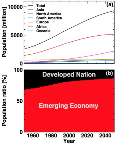
In 2013, United Nations announced that the world population exceeded 7.2

billion. The rising trend of the population is explosive, especially in China and

India. Figure 1.1 shows the evolution of the world population. In the future,

this rising trend will continue. Because of the population explosion, we are now

facing some problems, e.g., food distribution problem, environmental problem,

and energy problem. In particular, the energy problem is quite important,

since it can be connected with other problems such as environmental problem

or international peace issues. Figure 1.2 shows the history and prospect of the

world energy consumption, for developed nations and emerging economies, in

the unit of tone of oil equivalent (toe) [1]. In the near future, energy consump-

tion of emerging economies overtakes that of developed nations, having more

and more increase trend. Stable and economical energy source is strongly re-

quired from the emerging economic countries. It has been said that the recent

climate change in the world is so serious, because of extremely rapid consump-

tion of fossil energy resources. After the fission plant accident in Fukushima

in 2011, people’s way of thinking on the safety energy source became more

Fig. 1.1 (a) History and prospect of world population and (b) pop- ulation ratio between developed nations and emerging economies.

Data is quoted from population division of United Nations [www.un.org/en/development/desa/population/].

sensitive. Moreover, the fossil resources, and even nuclear fission resources are

limited. Scrambles of the limited resources provide not only destabilization

of the supply and their prices, but also international frictions, as is seen in

Middle Eastern countries. Renewable energies, e.g., solar power, wind power,

and hydroelectricity, are now gathering attention, and new business system on

the clean energy source is created depending on the government investments,

in some countries. However, their efficiency, economy, and stability are too

Fig. 1.2 History and prospect of world energy consumption [1].

Fig. 1.3 Cross sections for fusion reactions as a function of deuterium energy [2].

far insufficient to sustain the modern society. Considering keeping peaceful and sustainable society, we are now at turning point to reconstruct the world energy generation system.

Thermonuclear fusion reactor — exhaustiveless, safe, efficient and clean en-

ergy source — is going to be realized realizing owing to the great effort of sci-

entists and engineers all over the world [2]. There are several possible nuclear

reactions, i.e., deuterium and tritium (D-T) reaction, deuterium and deuterium

Fig. 1.4 Schematic illustration of the ITER [2].

(D-D) reaction, and deuterium and helium-3 (D-He

) reaction. Figure 1.3 shows the cross sections for these fusion reactions. As seen in the figure, the cross section of D-T reaction is more than 100 times larger than the other two reactions with the deuterium energy of under 100 keV. For the present, our first goal is to realize nuclear reactor using the D-T reaction. In order to make nuclear reaction, we need high-energy fuels, as shown in Fig. 1.3. In particu- lar, the nuclear reaction with high temperature fuels that thermal particles can induce nuclear reaction, i.e., temperature ∼ 10 keV, is called thermonuclear fu- sion. Note that the main reaction is carried out by particles in the Maxwellian tail so that the temperature is not needed to be as high as that corresponding to the energy of the maximum cross section. Thermonuclear fusion reactor is considered to be realistic in the economical and industrial aspects.

In the extremely high temperature, fuels are no longer the neutral gas, but

(ITER) is now under construction [3]. Schematic illustration of the ITER is shown in Fig. 1.4

Fusion energy is extracted through kinetic energies of neutron and α-particle.

Reaction equation is given as,

1

D

+

T

−→

He

+

n

, (1.1) where the kinetic energies of the neutron and alpha particle are 14.1 MeV and 3.5 MeV, respectively. The neutron has no electric charge, so that is not confined by the magnetic field. Energy of the neutron is used to heat water outside the fusion device, whose energy is converted to electric energy through the same way with nuclear fission reactor. Since the α-particle has electric charge, it is confined in the magnetic field like the fuel ions. This high energetic α-particle contributes to plasma heating through usual collision process in the confined plasma. The fusion energy gain factor Q is defined as,

Q = P

P

, (1.2)

where P

and P

are fusion energy and input energy, respectively. In order

to achieve enough high temperature plasma to induce fusion reaction, high

power heating system is required, such as electron and ion cyclotron resonance

heating, high-energy neutral beam injection, etc. Using the α-particle heating,

self-sustain plasma, i.e., high temperature plasma sustained only by the α-

particle heating with Q = ∞ , can be achieved. (For the first step, a target

Fig. 1.5 History of improvement of fusion triple product [2].

of the ITER experiment is Q = 10.) This process is sometimes mentioned as self-ignition. The self-ignition condition can be written as,

ˆ

nτ

T > ˆ 5 × 10

m

skeV, (1.3) where ˆ n, T ˆ , and τ

denote peak ion density and temperature, and energy confinement time respectively. This parameter is called as fusion triple product.

Therefore, our ultimate purpose to study plasma physics is to increase these three parameters by controlling plasma. Step-by-step increment of the fusion triple product can be seen in Fig. 1.5.

1.2 Plasma Confinement

Time evolution of plasma confined energy W

is often expressed as,

∂W

∂t = − W

τ

+ P

, (1.4)

where, W

is defined as,

W

≡

∫ 3

2 n(T

+ T

)d

x. (1.5)

prediction of τ

from plasma parameters is generally challenging. In steady state, Eq. (1.4) becomes,

W

= P

τ

. (1.7)

In order to increase plasma parameters, there are two ways, i.e., increasing P

by industrial effort, and increasing τ

by understanding and controlling plasma activity.

Historically, both directed efforts have been studied. Various heating sys- tems have been developed, and many physical findings have been discovered.

However, nonlinear properties of magnetically confined plasmas have made the

design of fusion device so complex. For example, when the input power P

is increased up to a certain level, unexpected decay of the energy confinement

time τ

is happened. Detailed measurements have revealed that the decay in

τ

is due to anomalous transport of the plasma, caused by micro-scale tur-

bulence [4–7]. In addition, further increment of P

has brought another un-

expected confinement stage, abrupt improvement of τ

, which is referred as

H-mode [8–10]. In the historical context, current common sense of the fusion

research in the world is that, fusion reactor relying on only industrial efforts

cannot be realized, because of the difficulty of the plasma control, as well as

the economic standpoint.

1.3 Approaches

The subject that the researchers in the world are shearing is, how to under- stand and control plasma activity. One of the key properties to understand the plasma activity is nonlinearity. As a result of nonlinearity, turbulence state is easily developed, and turbulent plasma becomes unpredictable matter. One of the goals of the physics of nonlinear plasma dynamics is to provide explanations to the anomalous transport and transitions to the H-mode and other improved confinement states. Since the micro-scale plasma turbulence is experimentally observed first, many works have been done to understand and control it. At the time, study on like-scale nonlinear interactions, which are seen in Kolmogorov’s cascade theory [11], or micro-scale turbulence evolution toward broad band spectrum [12], was focused on. Cause of anomalous transport was found in the micro-scale turbulence. For decades, in order to explain global and abrupt change in confinement state, multi-scale interaction, such as nonlinear interac- tion between micro-scale and meso- or macro-scale fluctuation, which involves structure formation has been intensely studied [13–15]. Difficulties in theoreti- cal modeling, numerical calculation and experimental prediction brought from nonlinearity have been overcome by the helps of novel diagnostics and exper- imental technique, as well as prodigious rapid-progress of powerful calculator.

The picture that the global flow structure excited by multi-scale interaction of micro-scale turbulence suppresses the micro-scale turbulence again by shear- ing effect, and stabilizes plasma confinement has been constructed. Prominent works are summarized in Chapter 2.

Now, the research is proceeded to the next stage. Former achievement was

based on long-time average to pursue statistical features of turbulence, and

cases of transit event like H-mode transition was excluded. In order to under-

stand this kind of transition event, analysis on the non-stationary phenomena is

experiments, namely time dependent parameter modulation experiments, are performed focusing on the purpose. As was pointed out by [17], the transient responses of turbulence and transport were found to be completely different from the conventional picture of stationary plasmas. In the standard view, the transport relation has been looked for in a form like q = − χ ∇ T . However, the new analysis has shown the hysteresis between mean gradient and mean flux, although the plasmas do not show transitions in confinement modes. In other words, the transport relation might be rewritten substantially in future. From both the industrial issue on realization of fusion reactor and academic issue on physics of complex systems, study on the transit event should be promoted.

1.4 Subject of This Thesis

Subject of this thesis is to promote extension of nonlinear plasma turbulence study from stationary state to non-stationary state. This thesis is organized as follows:

In Chapter 2, basis of plasma instability and turbulence, and turbulence transport are summarized. After that, achievements of multi-scale nonlinear coupling study performed in the world are reviewed. World trends of studies on plasma turbulence in the non-stationary state are also introduced.

In Chapter 3, the methods of the study are explained. In order to obtain

synthetic understanding of non-stationary turbulence activity, we use three

different devices, the JAERI Fusion Torus-2M (JFT-2M), the Large Helical

Device (LHD), and the Plasma Assembly for Nonlinear Turbulence Analysis (PANTA)/Large Helical Device (LMD-U), depending on targets. The expla- nations of each device and our targets are given. Principles of diagnostics that are used in this thesis, i.e., Langmuir probes, microwave reflectometory, Electron-Cyclotron-Emission (ECE) radiometer, and Heavy Ion Beam Probe (HIBP), are reviewed. Fundamentals and applications novel analysis methods, which are essential to observe the non-stationary state physics, i.e., short time Fourier transform, wavelet transform, Hilbert transform, and numerical filters, are explained.

Experimental results are shown from Chapter 4. There are three elements in our results, those are, dynamics in transport, in multi-scale interaction, and in transition phenomena, which are explained in Chapter 4, 5 and 6, respectively.

Chapter 4 provides new wavelet analysis method of heat pulse propagation experiment (explained in Chapter 2) that enables to obtain transport coefficient with fine temporal resolution [18]. The upper limitation of time resolution of the wavelet method is evaluated. Actual application of the method for the LHD heat pulse experiment is also given [19]. With the wavelet method, stochastic magnetic field structure is clearly observed.

In Chapter 5, we discuss spatiotemporal variation of nonlinear coupling

strength. In the first half, solitary wave-like turbulence observed in the LMD-

U experiment is analyzed with the wavelet bicoherence [20, 21]. From a local

measurement, a periodic oscillation of the bicoherence is observed, which is in-

terpreted as the spatial inhomogeneity of strength of nonlinear coupling. In the

last half, gradual temporal change of bicoherence and biphase, due to that in

background profiles is discussed for LHD [22]. In LHD, the low frequency fluc-

tuation that has long range correlation in the radial direction is observed. Time

evolution of the nonlinear coupling and nonlinear phase of the low frequency

mode, which result in distortion of waveform to nonsinusoidal signal, is ob-

evolution of transition front is observed. The speed of the transition front is found in the order of the ion sound speed. We discuss causality of transition by observing temporal evolution of mode power. At the transition, two modes, i.e., a mode traveling in the ion diamagnetic drift direction and a usual drift wave type mode, change first simultaneously, and other modes follow that of two modes. In the latter half, observation of a continuous transition and inverse transition event between L-mode and H-mode, so-called Limit-Cycle Oscillation (LCO), in JFT-2M is summarized [24]. The observation of the spatiotemporal structure of the electrostatic potential oscillation yields that there are no zonal flows, in contrast to the predator-prey model. The oscillation is found to be the periodic generations or decays of barrier with edge-localized mean flow.

Oscillatory Reynolds stress is found to be too small to accelerate the LCO flow, by considering the dielectric constant in magnetized toroidal plasmas.

Propagation of changes of the density gradient and turbulence amplitude into the core is also observed.

The important results of experiments are summarized in Chapter 7.

Review

Turbulence is spontaneously excited under various situations in non- equilibrium state plasmas, and governs plasma dynamics through nonlinear interactions. In this chapter, we first discuss the theoretical description of a drift instability, which plays crucial roles in the turbulent transport, and structure formations of magnetized plasmas. Next, we describe the transport process caused by fluctuations. Then, nonlinear effects of turbulence are explained. Finally, we review the recent studies of turbulence structure forma- tions in magnetically confined plasmas. The contents are based on [12, 25, 26]

for explanation in section 2.1-2.4.

2.1 Derivation of Dispersion Relation for Low Frequency Modes

Waves can be excited by free energy of plasmas. Spatiotemporal waveforms can be expressed as a superimposition of sinusoidal waves, called elementary wave components, that have frequency ω and wavenumber k. For example, a spatiotemporal wave propagation of the electrostatic potential can be expressed as,

φ(t, x) = ∑

ω,k

φ

= ∑

ω,k

φ

exp(ik · x − iωt), (2.1)

where x and t stand for the position vector and time, respectively. Equa- tion (2.1) is called Fourier decomposition of time series. Generally, only the waves having specific combination of (ω, k) are allowed to exist in materials and/or fields. This combination can be written as,

ω = ω(k), (2.2)

and is called the dispersion relation. The dispersion relation can be derived from a set of equations that governs dynamics of the materials and fields, as an eigenvalue of the equations. For example, the dispersion relation of a wave of electric field and magnetic field in vacuum, i.e., light, can be derived from Maxwell’s equations as ω = ck, where c is the speed of light in vacuum.

The dispersion relation is one of the standard information of wave, therefore, investigation of the dispersion relation is the first step for the study of plasma turbulence.

Low frequency waves are focused on in this section because they have a capability to convey plasma particles with violation of the magnetic confinement (see the following section for details). Here, fluid description of the plasma is applied to derive the dispersion relation. The dispersion relation is derived from the equations of plasma dynamics (continuity equation and equation of motion), equations of electromagnetic fields (Maxwell’s equations), and thermodynamic equation (equation of state). The continuity equation and equation of motion are,

∂n

∂t + ∇ (n

· v

) = 0, (2.3)

m

n

dv

dt = −∇ p

+ e

n

(E + v

× B), (2.4) where, n

, v

, m

, p

, and e

stand for the density, velocity, mass, pressure, and electric charge of each species expressed by the suffix j, respectively, and

d

dt = ∂

∂t + v · ∇ (2.5)

∇ ·

j

∇ · B = 0, (2.9)

where E and B are the electric field and magnetic field, respectively.

The equation of state is widely used to close the set of equations. On one hand, when the adiabatic condition is satisfied, the relation

d(p

n

)

dt = 0, (2.10)

can be used, where γ

is the specific heat ratio. On the other hand, under the iso-thermal condition,

dT

dt = 0, (2.11)

can be used.

Thus, the set of equations is partial derivative nonlinear equation, so that it is too complicated to solve generally. An assumption that the fluctuation amplitude is much smaller than the mean value is reasonable to proceed further, as a first step. (Of course, the nonlinear terms make the plasma physics difficult, and many works are dedicated for this topic.) If the variables can be expanded as

n = n

+ ˜ n, (2.12)

v = v

+ ˜ v, (2.13)

E = E

+ ˜ E, (2.14)

.. .

where the terms with suffix 0 and tilde represent the mean part and perturba- tion part, respectively, and the quadratic perturbation terms can be neglected.

This is called linearization of the equations, and it can reject nonlinear terms and makes the set of equations linear.

In addition, since we assume Fourier decomposition with harmonic oscillation for the variables as shown in Eq. (2.1), time and spatial derivative terms can be rewritten as,

∂

∂t → − iω,

∇ → ik. (2.15)

Using the linearization and Fourier decomposition, the partial derivative non- linear equation becomes linear algebraic equation, which can be easily solved.

Because of the elimination of the nonlinear terms, the set of equations can be separately solved for each combination of (ω, k). Otherwise, cross terms of Fourier series appear, and all equations for any combination of (ω, k) are directly connected.

In the low frequency fluctuation satisfying the relation

(ω/k)

v

, (2.16)

where v

indicates the electron thermal velocity. Electrons can almost freely respond to the electric field fluctuation if there is no effect of magnetic field.

The electrons move to the equilibrium position within a very short time when the electric field changes. The relation Eq. (2.16) allows us to eliminate the inertia term in the equation of motion for electrons in the parallel component to the magnetic field.

We are also interested in a situation where the scale-length of fluctuation is

much longer than the Debye length, kλ

1. Then the quasi-neutral condition

2.2 Linear Excitation Mechanism of Drift Wave

The drift wave is excited if there is an inhomogeneity of density perpendicular to the magnetic field line. In this section, we first derive the dispersion relation of the ion sound wave without the inhomogeneity of the density. Then the gradient of density is taken into account and the dispersion relation of the drift wave is derived. The resistivity of the plasma that makes the drift wave unstable is considered in the last subsection of this section.

2.2.1 Ion Sound Wave

In this subsection, the mean profile of plasma is assumed to be uniform, stationary and having cylindrical symmetry with the stationary magnetic field in the axial direction. We use cylindrical coordinates (r, θ, z), and have

∇ n

= 0, v

= 0, E

= 0, B

= (0, 0, B). (2.18) We consider a situation that the wave propagates in the direction parallel to the magnetic field with the electrostatic potential fluctuation ˜ φ,

k = (0, 0, k

), (2.19)

E ˜ = −∇ φ. ˜ (2.20)

The frequency is considered to be in the range,

| k

v

| ω | k

v

| . (2.21)

Then, the ion response is assumed to be adiabatic, and the electron response is considered to be iso-thermal.

We start to derive the dispersion relation from the equation of motion for ions,

− im

n

ω ˜ v

= − ik

e

n

φ ˜ − ik

p ˜

. (2.22) The continuity equation for ions,

− iω˜ n

+ ik

n

v ˜

= 0, (2.23) is used to eliminate ˜ v

, and we obtain,

˜ n

n

= (

1 − k

ω

γ

T

m

)

k

ω

T

m

e φ ˜

T

, (2.24)

where we take the charge number of ions as unity and the adiabatic condition (2.10) is employed. The equation of motion for electrons is written by neglecting the inertial term as,

ik

en

φ ˜ − ik

p ˜

= 0. (2.25) The iso-thermal condition of electrons gives the relation ˜ p

= T

n ˜

, by which Eq. (2.25) is rewritten as,

˜ n

n

= e φ ˜

T

. (2.26)

This relation is often called Boltzmann’s relation. We can close the Eqs. (2.24) and (2.25) by the help of quasi-neutral condition [Eq. (2.17)], and obtain the dispersion relation as,

ω

= c

k

, (2.27)

where c

is the ion sound velocity given by, c

= T

+ γ

T

m

. (2.28)

Fig. 2.1 Propagation of ion sound wave.

If the ion temperature is much smaller than the electron temperature (T

T

), the ion sound velocity becomes,

c

= T

m

. (2.29)

The ion sound wave is generated by an expansion of ions in a high density layer to a low density layer, which is conducted not only by the pressure of ions but also by the electric field, as is displayed in Fig. 2.1. Free electron motions parallel to the magnetic field is the key physics of the propagation of the ion sound wave.

2.2.2 Drift Wave

The density gradient perpendicular to the magnetic field line induces the drift wave. We take the density gradient in the r direction, and the propagation direction in the θ and z directions as,

k = (0, k

, k

). (2.30)

A new term appears in the continuity equation due to the radial density gradient and Eq. (2.23) is modified as,

− iω n ˜

+ ik

n

v ˜

+ dn

dr v ˜

= 0. (2.31) The radial component of the equation of motion for ions provides,

˜

v

= − ik

φ/B. ˜ (2.32)

The equation of motion in the parallel direction does not vary from Eq. (2.22).

Elimination of ˜ v

and ˜ v

[by use of Eq. (2.22) and Eq. (2.32)] from Eq. (2.31) gives the ion density fluctuation in terms of the potential perturbation as,

˜ n

n

= (

1 − k

ω

γ

T

m

)

( k

ω

T

m

− 1

ω k

T

eB 1 n

dn

dr

) e φ ˜ T

. (2.33)

The motion of electrons is described by the Boltzmann’s relation in Eq. (2.26).

Substitution of Eq. (2.33) and Eq. (2.26) into the quasi-neutral condition Eq. (2.17) gives the dispersion relation as,

ω

− ωω

− c

k

= 0, (2.34) where ω

is the drift frequency defined by

ω

= k

T

eB 1

L

= v

k

, (2.35)

where v

is called the electron diamagnetic velocity. The term L

in the Eq. (2.35) is called the scale length of density gradient and is defined as,

1

L

= − 1 n

dn

dr . (2.36)

When the wave propagates almost in the θ direction satisfying, ρ

L

> | k

|

| k

| , (2.37)

Fig. 2.2 Propagation of drift wave [25].

where ρ

= v

m

/eB denotes Larmor radius of ions, the relation v

k

c

k

is held. The dispersion relation Eq. (2.34) becomes,

ω = ω

. (2.38)

Geometry of the drift wave propagation in the cylindrical coordinates is

shown in Fig. 2.2(a). Since there are two directions of propagation in Eq. (2.35),

the constant density surfaces become helically twisted shape. Figure 2.2 (b) is

the cross section of the cylindrical plasma that is illustrated by the rectangular

domain in Fig. 2.2 (a). If there is a finite wavenumber in the θ direction as

shown in Fig. 2.2 (b), the inhomogeneity of the density appears due to the sta-

tionary density gradient in the r direction. The motion of the freely movable

electrons makes the Boltzmann’s relation, hence the fluctuation of the electric

field in the z direction is excited. The E × B convection in Eq. (2.32) gives

the motion in the r direction with the π/2 of the phase delay with respect to

the ˜ φ. The radial motion realizes the motion of equi-density contour in the θ

direction. Thus the drift wave propagates in the θ direction.

2.2.3 Resistive Drift Wave

If the dissipation of plasma (e.g., resistivity, electron Landau damping, etc.) is taken into account, the Boltzmann’s relation is modified. The dissipation impedes the free motion of electrons, then Eq. (2.26) becomes,

˜ n

n

= (1 − iδ

) e φ ˜ T

, (2.39)

where δ

is the delay of the electron density response from the potential fluc- tuation. If the imaginary part of the frequency (δ

) is positive, the oscillation amplitude grows exponentially. We estimate the sign of δ

by considering a small but finite collision of electrons as dissipation. The small friction term

− m

n

ν v ˜

is added in the equation of motion for electrons, and Eq. (2.25) is modified as,

ik

en

φ ˜ − ik

p ˜

= m

n

ν v ˜

. (2.40) The continuity equation for electrons is adopted to eliminate the term ˜ v

as the same procedure for ions, and finally,

˜ n

n

=

(

1 + i ν(ω

− ω) k

v

)

e φ ˜ T

'

(

1 − i ν(ω

− ω) k

v

) e φ ˜

T

, (2.41) is obtained. Therefore, the delay δ

is expressed as,

δ

= ν(ω

− ω)

k

v

. (2.42)

The dispersion relation Eq. (2.34) becomes,

ω

− ωω

− c

k

+ iδ

(ω

− γ

k

v

) = 0, (2.43) In the limit of | δ

| 1 and v

k

k

c

, Eq. (2.38) is modified as,

ω = ω

(1 + iδ

). (2.44)

∼

ii) The amplitudes of the normalized electron density fluctuation and nor- malized potential fluctuation are almost the same as,

n ˜

n

∼

e φ ˜ T

. (2.45)

iii) The waveform of the electron density fluctuation and potential fluctu- ation are similar, and the phase difference between them is small (the phase delay of the density from the potential has to be positive.).

iv) The wavenumber of the electron density fluctuation or potential fluctu- ation in the z direction is finite (shown in Fig. 2.2 (a)).

2.3 Transport by Fluctuation

If there is the radial transport of particles and energy, the change of den- sity and temperature at the plasma core is induced. The study of the radial transport has been mandatory. In this section, the physics of the transport due to electric field fluctuations is illustrated in comparison with the collisional transport.

2.3.1 Transport by Collision

Once a particle experiences a Coulomb collision, its orbit is changed. Since

the radial transport appears in the direction across the field line, the particle

can move with a step up to the gyro radius ρ

per one collision in homogeneous magnetic field. If collisions occur with the frequency ν

, particles diffuse with a diffusion coefficient of

D

' ν

ρ

, (2.46)

where the suffix c indicates Coulomb collision.

2.3.2 Transport by Electric Field Fluctuation

The electric field fluctuation is generated by various mechanisms, e.g., by excitation of the drift wave. The fluctuation of the electric field that has the frequency lower than the ion cyclotron frequency makes the E × B convection fluctuation in plasma as,

V ˜

=

E ˜ × B

B

. (2.47)

In the diffusion process, variance of radial position of particles ˜ r(t) is propor- tional to the time t with the coefficient D as,

h{ r(t) ˜ − r(0) ˜ }

i = Dt. (2.48) Since the electric field fluctuation can be expressed by use of the Fourier de- composition [Eq. (2.1)], the time evolution of the fluctuating radial position (owing to a sinusoidal wave) can be estimated as,

˜

r(t) − r(0) ˜ ' iE

(ω − k

v

+ iν)B exp(ik · x − iωt), (2.49) with the approximations that the motion along the field line is unperturbed and the perpendicular wavelength is much longer than ˜ r(t) − r(0). We consider ˜ a small decorrelation ν around the resonance at ω − k

v

= 0. The deviation in the radial direction per each period becomes the amplitude of the fluctuation of the position as,

∆

= E

(ω − k

v

+ iν)B . (2.50)

proportional to the squared amplitude of the electric fluctuation as, D ∼ 1

τ

( E

B )

. (2.52)

When the fluctuation amplitude is large, ∆

reaches comparable to the perpendicular wavelength k

. In this case, the correlation time of fluctuation field that resonant particles feel is limited by τ

≤ k

(E

/B)

. Substituting this (crude) estimation into Eq. (2.52) gives

D ' 1 k

E

B . (2.53)

The diffusion coefficient becomes a linear function of the fluctuation ampli- tude under the strong turbulent condition. Turbulence amplitude is directly connected with transport.

2.4 Nonlinear Effect of Turbulence

Plasma in the turbulent state contains various waves that may be decom-

posed into terms of elementary wave components with various wavenumbers

and frequencies. In order to study nonlinear process, the mutual interaction of

the waves with different wavenumbers and/or frequencies should be took into

account. Here, we briefly explain the nonlinear energy cascade process and the

effect of the nonlinearity on the transport coefficient. Then, we introduce the

effect of disparate scale interaction.

2.4.1 Energy Cascade and Dissipation

Here we discuss the energy cascade process in turbulence by taking an ex- ample of neutral fluid theory. The electromagnetic force term in Eq. (2.4) is neglected and Navier-Stokes equation with incompressibility of velocity is used as,

mn dv

dt = −∇ p + µ ∇

v, (2.54)

where µ is the viscosity of the fluid. The energy spectral equation is derived from Eq. (2.54) as,

∂E (k)

∂t = − 2(µ/mn)k

E(k) + T (k), (2.55) where E(k) and T (k) are the energy spectrum and the spectral energy transfer rate by nonlinear interactions, respectively. The energy spectrum is defined as,

E(k) = 2πk

h v

(k; t)v

(k

; t) i

δ(k + k

) , (2.56)

where the denominator and numerator in the right side of Eq. (2.56) are the two-point correlation of the velocity field expressed by wavenumber and delta function, respectively. The suffix in the numerator is the vector subscript. The integral of the energy spectrum over k gives the energy of turbulence K as,

K =

∫

0

E(k)dk. (2.57)

The spectral energy transfer rate T (k) in Eq. (2.55), which is a cubic correlation

of the velocity, expresses the energy exchange rate of the mode that has the

wavenumber k, by the interaction with modes that have the wavenumbers p

and q. T (k) contains δ(k − p − q), i.e., the mode can interact only with the

modes that satisfy k = p + q. The spectral energy transfer rate comes from

the nonlinear convection term in Eq. (2.54). When fluctuations are excited in

0

T (k)dk = 0. (2.58)

One can derive the equation for the energy of turbulence K from Eqs. (2.56)- (2.58) as,

∂K

∂t = ≡ −

∫

0

D(k)dk, (2.59)

where is the dissipation ratio and D(k) is the dissipation spectrum written by

D(k) = 2(µ/mn)k

E(k). (2.60)

The squared wavenumber k

makes the dissipation spectrum large in small scale (large wavenumber region) and small in large scale (small wavenumber region).

If there is a large separation between the maximum scale and minimum scale of the turbulence, the spectral separation between E (k) and D(k) becomes large.

A scale region between the peaks of E(k) and D(k), where one can regard as independent from the energy injection or dissipation, is called inertial region.

The spectral energy flux Π(k) is defined by T (k) = − ∂Π(k)

∂k , (2.61)

where,

Π(k) = −

∫

T (k)dk =

∫

k

T (k)dk (2.62)

is held. The spectral energy flux Π(k) stands for the energy transferred from the

smaller region to larger region than k. In stationary inertial region, Eq. (2.55)

Fig. 2.3 Conceptual diagram of energy spectrum E(k) and energy dissi- pation spectrum D(k) [26].

Fig. 2.4 Conceptual diagram of spectral energy transfer rate T (k) and spectral energy flux Π(k) [26].

becomes,

∂E (k)

∂t = T (k) = − ∂ Π(k)

∂k = 0, (2.63)

and Π(k) = const.(= ) is held. Then the energy spectrum can be written by use of only k and as,

E (k, ) ∝

k

. (2.64)

The indices α and β are determined only by the dimensions of E, and k. The

diagrams of the relation between E(k) and D(k), and the relation between T (k)

and Π(k) are shown in Figs. 2.3 and 2.4, respectively. An image of the cascade

Fig. 2.5 Image of cascade and dissipation [26].

and dissipation is shown in Fig. 2.5.

2.4.2 Dressed Test Mode and Nonlinear Diffusion Coefficient

Effect of nonlinearity to the transport coefficients can be analyzed by the method of dressed test mode. Equation system that describes instability can be written as,

{ ∂

+ L } f = N , (2.65)

where ∂

, L, f and N are the linear operators related to the time derivative, the matrix of linear operators, the perturbed field (e.g., the electric potential, the pressure), and the nonlinear terms. The diagonal elements of the linear operator contain the dissipation terms, for example, the collisional diffusion coefficient µ

. The nonlinear terms come from the nonlinear convection term of Lagrange derivative.

We consider the nonlinearity of a test mode k with background turbulence k

as shown in Fig. 2.6. The nonlinear term N is treated using the renormalization

method as following. The interaction between the test mode and background

turbulence generates a driven mode k

. If the driven mode interacts with

Fig. 2.6 Screening by the background turbulence.

Fig. 2.7 Interaction of a test mode with a background turbulence and back-interaction to the test mode [12].

the background turbulence, the generated mode contributes to the test mode, which is called the back-interaction. Calculation of the back-interaction gives the description of the direct interaction of the test mode with the background turbulence. This procedure is shown in Fig. 2.7.

Some approximation methods help to solve Eq. (2.65) and the dressed test mode

{ ∂

+ ¯ L } f = 0 (2.66)

Eqs. (2.66) and (2.67). The marginal stability condition for the dressed test mode is considered as the eigen-equation that determines µ

. The nonlinear dissipation terms are written as a function of the amplitude of the background turbulence. Therefore, the fluctuation level and intensity of transports of particles and energy are deduced.

2.4.3 Disparate Scale Interaction

In the former two subsections, we have discussed nonlinear effects in the fluctuations that have similar temporal/spatial scales. However, especially in the magnetic confined plasmas, there are various distinct scale lengths, e.g., electron and ion gyroradii, Deby length, and scale length of gradient. Plasma dynamics can be at each of the scales, so that the dynamics of entire plasma is governed by the multi-scale dynamics and their interconnection. This intercon- nection is called disparate interaction [27]. If there are two kinds of fluctuations with different scales, i.e., one having the high-frequency and small spacial scale (large wavenumber) and the other having the low-frequency and larger spatial scale (small wavenumber), the fluctuation with the large wavenumber can act as a pressure that induces the fluctuation with the small wavenumber as illus- trated in Fig. 2.8 (a). In Fig. 2.8 (a), two large wavenumber modes k

and k

directly drive a small wavenumber mode q by, e.g., parametric instability.

This process completely differs from (inverse) cascade process, as illustrated in

Fig. 2.8 (b). In the system of the disparate interaction, the fluctuation with

small wavenumber can strain that with large wavenumber.

Fig. 2.8 Wavenumber relation among different scale fluctuations in (a) disparate scale interaction and (b) inverse cascade [27].

An important example of the system of disparate scale interaction observed in magnetized confined plasma is drift wave (large wavenumber)-zonal flow (small wavenumber) system. The reason for which the system is important for plasma confinement is that the zonal flow can regulate the turbulence transport excited by drift wave turbulence (experimental observation of the zonal flow is given in the next section). Zonal flow shear can stretch and elongate the eddy of drift wave turbulence in the poloidal direction as illustrated in Fig. 2.9.

This stretch shortens the radial wavelength (the wavelength is proportional to

the eddy size) of the drift wave. As a result, typical step size of turbulence

transport is reduced, or, the transport coefficient is reduced via the increase of

the radial wavenumber as shown in Eq. (2.53). The schematic illustration of

drift wave-zonal flow system is shown in Fig. 2.10.

Fig. 2.9 Shearing of drift wave eddies by zonal flow [27]. black circles and ellipses show eddies of drift wave and blue arrows shows E × B flow induced by zonal flow fluctuation.

Fig. 2.10 Schematic illustration of drift wave-zonal flow system [27].

2.5 Recent Experimental Achievement on Multi-Scale Interaction

Recently, many theoretical and experimental works are focused on nonlin-

ear process, especially on multi-scale turbulence interaction [28]. Micro-scale

plasma turbulence, which has broad band incoherent fluctuation spectrum in both frequency and wavenumber space, is normally excited by instabilities with extremely complex nonlinear process. Saturated turbulence sometimes excites meso-scale or macro-scale fluctuation, accompanied with global structure of parameters, e.g., flow or density. In this section, we introduce the latest ex- perimental observations of multi-scale coupling, which result in structural for- mations in plasma. The phenomena are regarded as quasi-stationary, and the analyses are based on long time average. The nonlinear coupling of turbulence is surveyed by using bispectral analysis.

2.5.1 Zonal Flows

One of the most exciting results of nonlinear process in confined plasmas

might be zonal flows. Zonal flow is a band-like shear flow observed not only

in the magnetic confined plasma, but also in the universe, e.g., striped pattern

on the surface of Jupiter shown in Fig. 2.11. Illustration of the zonal flow in

the poloidal cross section of magnetic confinement toroidal plasma is shown

in Fig. 2.12. The zonal flow is regarded as a key to realize the thermonuclear

fusion because it has a potential to prevent turbulent transport phenomena

[13–15, 28]. It was discovered in compact helical system (CHS) in 2004 for the

first time, by direct electric potential fluctuation measurement using two heavy

ion beam probes (HIBP) [30]. The band-like flow structure was characterized

by toroidal and poloidal mode number n and m, as n = m = 0, with finite

wavelength in the radial direction. Figure 2.13 shows the time evolution of

the potential fluctuation in different toroidal positions indicated by red and

blue curves. If the radial positions are the same, the waveforms are similar [as

shown in Fig. 2.13 (a)]. However, signals from the different radial positions

have a finite phase difference [as shown in Fig. 2.13 (b)]. In addition, the radial

structure of zonal flow was measured with two-point correlation technique as

Fig. 2.11 Zonal flow on Jupiter obtained by Hubble Space Telescope (HST) [29].

Fig. 2.12 Illustration of zonal flow in magnetic confined plasma. Arrows denote directions of plasma flow.

shown in Fig. 2.14. One measurement point was altered in the radial position,

which is represented by the horizontal axis in Fig. 2.14, while the other was

fixed at r = 12 cm. A sinusoidally changing structure indicates the finite

wavelength. The existence of zonal flow and internal transport barrier (ITB)

was also demonstrated. Figure 2.15 shows the change of zonal flow amplitude

with and without ITB. The solid line in Fig. 2.15 indicates the transition time.

Fig. 2.13 Time evolution of zonal flow [30].

Fig. 2.14 Radial structure of zonal flow [30]. Cross correlation coefficient (closed circles) and coherent structure of fast Fourier transform (opened circles) are shown.

The zonal flow amplitude decreases after the back transition. In addition, the amplitude of density fluctuation increases at the same time. This observation demonstrates the suppression of turbulence by zonal flow.

The excitation mechanism of the zonal flow was predicted in terms of nonlin-

ear modulational coupling of turbulence. The nonlinear coupling between zonal

flow and background turbulence was observed by bispectral analysis, which is a

Fig. 2.15 Zonal flow with and without a transport barrier [30]. Time evolution of (a) density fluctuation and (b) zonal flow potential gradient fluctuation. Solid vertical line indicates the transition time.

powerful tool to investigate the strength of nonlinear coupling (see chapter 3 for details). Figure 2.16 shows the variation of squared wavelet bicoherence (also see chapter 3.) with the fluctuating zonal flow potential. When the zonal flow potential becomes the minimum or maximum, the nonlinear coupling between zonal flow and the turbulence appears strongly.

Although the existence of nonlinear coupling was demonstrated by bispec-

tral analysis, the causal relation between zonal flow and turbulence had been

difficult to clarify. To overcome this difficulty, Camargo method [32] was ap-

plied to the zonal flow in TJ-K [33]. To identify the energy flow direction,

i.e., whether the energy flows from turbulence to the zonal flow or vice versa,

wavenumber vector of turbulence has to be measured. This is because nonlin-

ear energy transfer is carried out by convective term in the equation of motion,

(v ·∇ )v, through so-called Reynolds stress. Velocity field in the plasma is given

by E × B velocity, where E = −∇ φ = − kφ. In TJ-K, turbulence fluctuation

Fig. 2.16 Nonlinear coupling of zonal flow. Strength of nonlinear coupling varies with fluctuating zonal flow potential. Bicoherence diagram (a) when the potential is the maximum, (b) when the potential is between the max- imum and the minimum, and (c) when the potential is the minimum [31].

and wavenumber vector were measured with two-dimensional matrix probe ar- ray (8 × 8 on cross section of torus plasma) shown in Fig. 2.17. Figure 2.18 shows the computed energy transfer function. As mentioned above, nonlinear energy transfer, especially three-wave coupling process, only occurs among the wavenumber combination, k

, k

and k

, where they satisfy the wavenumber matching condition, i.e., k

= k

± k

. Figure 2.18 takes k

and ± k

in the horizontal and vertical axes, respectively. Red contour color indicates that the wave having k

is obtaining energy from those having k

and k

, while blue contour color indicates the energy loss of the wave with k

. This contour and overlapped total energy income indicate low frequency oscillation, which is mentioned as zonal flow, gains energy from turbulence.

Detailed physics of zonal flow can be studied on linear magnetized plasmas.

The zonal flow was also observed in LMD [35, 36] by use of floating potential

measurement with Langmuir probe array. Figures 2.19 (a) and (b) are the

radial profiles of the power spectra of the normalized floating potential and