電気通信大学学術機関リポジトリ

(1)

Computational theory of occluded-occluding

object perception in early visual cortex

Zaem Arif bin Zainal Abidin

Graduate School of Information Systems

The University of Electro-Communications

Tokyo, Japan

A thesis submitted for the degree of

Doctor of Engineering

(2)

Computational theory of occluded-occluding

object perception in early visual cortex

Examining Committee

Main Academic Adviser : Assoc. Prof. Shunji Satoh

Academic Adviser : Prof. Yutaka Sakaguchi

Academic Adviser : Prof. Takashi Suehiro

Examiner : Prof. Yoshiki Kashimori

(3)

Copyright © 2018 by Zaem Arif bin Zainal Abidin

All Rights Reseved

(4)

概要

外界には奥行きが異なる物体が多数存在し，これら物体の視覚情報は重なりっている場合が多い．このとき「遮蔽物体と被遮蔽物体を隔てる境界（Border）は遮蔽物体に帰属する」．Border Ownership（BO）問題は，物体の重なり順序を計算するための基盤的問題である．本研究の具体的な成果として，境界の Owner が存在する方向である BO 信号をベクトル場𝑬(𝑥, 𝑦)，重なり順序をスカラー場 𝜙(𝑥, 𝑦)として見なせば，電磁気学の電位と電場に関する定理（電場は電位の勾配，𝑬(𝑥, 𝑦) = 𝛁𝜙(𝑥, 𝑦)である）を用いることで問題の定式化ができることを発見した．数値シミュレーション結果から，提案モデルは様々な遮蔽状況や形状の変化に対して頑健に，BO 問題と重なり順序計算問題が解けることを見出した．

(5)

Abstract

Humans can distinguish the order of mutually overlapping objects in a visual scene. The border between an occluding object and the occluded object is “owned” by the occluding

object. How the brain assigns these borders, or Border-ownership (BO) assignment, determines the perception of object depth order. Findings from physiological experiments reveal that some neurons in area V2 of the brain respond selectively when the object which “owns” the edge in its receptive field is located on a specific side. Several models

have been proposed in existing studies to reproduce this phenomenon. However, these models are not based on a clear computational theory.

This study is the first to approach BO assignment from a computational viewpoint by treating it as a well-defined problem. I propose that the direction of BO assignment can be defined as a conservative vector field 𝑬(𝑥, 𝑦) with arrowheads pointing towards the occluding object, and that information pertaining to depth order can be defined as its corresponding scalar field 𝜙(𝑥, 𝑦). By using a theorem in electromagnetics which states that the gradient of electric potential is its electric field 𝐸(𝑥, 𝑦) = 𝛁𝜙(𝑥, 𝑦) , I demonstrate that the BO assignment problem can be solved by updating an initial vector field until its rotation, or “curl”, is zero.

(6)

A model developed on this computational theory can simultaneously reproduce BO assignment and perceived depth order. Results of numerical simulations agree qualitatively with the response of object-side selective neurons in V2 to stimuli containing occlusion with simple geometry. Neural networks can be deduced from the update rule curl using only one parameter for adjusting the scale of neural connections. This study also presents new interpretations of existing models in addition to insight into a possible method for calculation of depth order.

(7)

Acknowledgements

I would like to acknowledge and thank everyone who has supported me throughout the production of this thesis.

Firstly, I am greatly thankful to my academic adviser, Associate Professor Shunji Satoh for his guidance, patience and enthusiasm. Without his support, writing this thesis would not have been possible.

I would also like to express my gratitude to Professor Yutaka Sakaguchi for his invaluable advice, as well as Professor Takashi Suehiro, Professor Yoshiki Kashimori and Associate Tomohiro Ogawa for their insightful opinions.

In addition, I would also like to thank to everyone in the Laboratory for Human Informatics for their support and advice.

Last but not least, I would like to thank everyone in my family and extended family who provided me with encouragement and support thought my years in Japan.

(8)

1 Introduction

1.1 Background

1.1.1 Occlusion and object perception

Humans can identify and recognize objects with ease from a cluttered scene in their surrounding environment. Figure-ground organization, or the separation of an object from the rest of the image, is thought to be a preliminary process for cognition. Figure 1.1a shows an image referred to as “Rubin’s vase”, which illustrates the basis of figure-ground organization [1]. The image is perceived in two distinct ways. It is perceived as a vase if the light-grey region is treated as the “figure”, and the dark-grey region is considered as the “ground”. In contrast, the viewer perceives the image as two faces if the dark-grey region is considered as the “figure” and the light-grey region is considered as the “ground”.

Evidence for figure-ground organization is most apparent for a single object occluding a background. However, the real world is filled with several objects of various shapes and sizes, many of which mutually overlap one another. Figure 1.2 shows a photograph with several objects, some of which are occluded. There are several “figures” in this scene, and figure-ground organization only describes the separation of one figure at a time. To accurately grasp the relative location and nature of objects in a scene, one needs a sense of the order that obejcts are located in front of us: object “depth order”. Figure-ground organization would involve segregating these objects one at a time, starting from the plastic bottle in the foreground occludes the laptop. In contrast, assigning larger depth order values to objects closer to the viewer would allow an instantaneous grasp of how objects are placed before us in a visual scene.

(11)

adopted by the brain to approach problems in visual perception related to overlapping objects [2]. In a situation where one object occludes another, the border between them is “owned” by the occluding object. Let us revisit the example of Rubin’s vase in Figure

1.1 to see how BO assignment effects perception. The direction of BO assignment is

expressed by arrows pointing towards the occluding object along the perimeter of the border. In the perception of a vase, the border is owned by the inner region, as indicated by the arrows. Similarly, outward-pointing arrows imply that the border is owned by the two faces. For a real-world example, take a look at the plastic bottle in the foreground in

Figure 1.2. The border between the plastic bottle and the laptop computer is owned by

the plastic bottle. This border describes the shape of the plastic bottle. Conversely, this border is not owned by the laptop computer; part of the laptop computer is occluded by the plastic bottle, and the border between them does not describe the shape of the laptop computer. It is clear that BO assignment is important for the perception of object shape, as observed by psychologists [2]. However, does the human brain actually carry out BO assignment?

(12)

Figure 1.1 Bi-stable perception of Rubin’s vase.

The image in (a) can either be perceived as a (d) vase over a dark grey background or (e) two faces over a light grey background. BO assignment is believed to account for these two percepts. The direction in which borders are assigned to occluding regions dictates how the image is perceived. Arrows along the border perimeters point either towards (b) the inner or (c) the outer region, resulting in the perception of (b) a vase or (e) two faces, respectively.

(13)

Figure 1.2 A real-world example, where several objects mutually overlap.

Figure-ground organization does not adequately explain the perception of a scene where multiple “figures” exist. For example, the plastic bottle occludes the laptop computer, which occludes a jar. The order in which these objects overlap, or “depth order”, is important to gauge the nature of how objects are located in front of us. The border between the plastic bottle and the laptop computer, shown in red is owned by the plastic bottle. This means that the border describes the shape of the occluding plastic bottle, and not of the occluded laptop.

(14)

1.1.2 The human visual system

The human visual system processes information in a hierarchical manner. Local information such as luminance, color, and motion, are extracted from retinal images then subsequently integrated for a contextual understanding of the external world. A neuron in the visual cortex can only process information presented to it in a fixed range, located at a fixed location in the retinal image. This is the neuron’s “receptive field”. Figure 1.3 shows the flow of information between areas in the visual cortex as compiled and organized from past findings [3]. Each area of the visual cortex carries out a different processing task. For example, neurons in area V1 respond selectively to discontinuities in luminance, at a specific orientation, placed in their receptive field [4]. This supports the assertion that one task of area V1 is to extract edges from an image, some of which coincide with object borders. More complex tasks are conducted higher up in the hierarchy; research shows that area IT is involved with recognition [5].

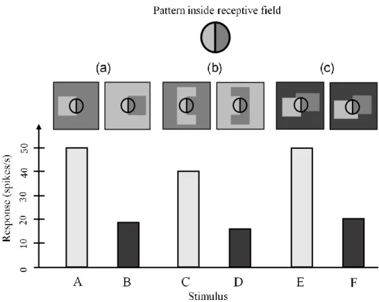
Physiological experiments revealed the existence of neurons in area V2 which respond strongly to an edge of an arbitrary orientation when an object is located on a specific of its receptive field: BO is coded in area V2 [6]. The emergence of BO signals were fast (30 ms after response onset), and latency was independent of object size [7]. Their experiments were conducted on monkeys using 2D images consisting of simple shapes such as single squares, C-shapes, and occluding rectangles. Figure 1.4 shows data of the response of a neuron in area V2 with a left-side object selectivity. The pattern in its receptive field, a 90-degree vertical edge, is the same for all stimuli. This implies that visual information outside of the neuron’s receptive field modulates its response. The response of a substantial subset of these BO-coding neurons were consistent with object-side even for complex natural scenes [8]. In addition, some BO-coding neurons also

(15)

respond selectively to three-dimensional (3D) objects in stereoscopic stimuli [9]. This implies that neurons in V2 utilize both global edge information and binocular depth information in BO coding to represent objects in a 3D space.

Area V4 may be the visual area where depth order is calculated. Some neurons have been reported to respond selectively to surfaces of various shapes [10]. Shape-selective neuron will respond selectively to an object of a specific shape if it is the occluding object [11]. Some neurons in area V4 have been shown to respond to subjective surfaces [12]. Lesions in area V4 also have been reported to impede the perception of color, brightness, shape, as well as subjective contours in monkeys [13], [14].

(16)

Figure 1.3 Hierarchical nature of visual processing in the brain.

Each area carries out a different visual processing task. Lower-level areas such as V1 extract local edges from retinal images for further processing. Area V2 is believed to be involved in BO assignment. Area V4 is involved with color, shape and surface perception. Area IT, located higher in the hierarchy is involved with object and face recognition.

(17)

Figure 1.4 Response of a neuron in area V2 towards pairs of stimuli demonstrates its object-side selectivity.

The receptive field of the neuron is represented by a circle, enlarged for explanatory purposes. The pattern inside the receptive field is the same for all cases: a vertical (90 degree) edge. (a) This neuron responds stronger towards stimulus A, where an object exists on the left side of its receptive field. In contrast, an object does not exist on the left side of the neuron’s receptive field in stimulus B. (b) Similarly, the neuron responds stronger to stimulus C than to stimulus D, and (c) stronger to stimulus E than to stimulus F. For all three cases, an occluding object exists on the left side of the neuron’s receptive field. Data was adapted from Zhou et al. (2000) [6].

(18)

1.1.3 Marr’s framework of visual processing

Marr (1982) proposed a framework of visual processing [15]. He argued that the processing of visual information is carried out in four distinct stages:

(1) Visual information from the external world is projected as two-dimensional images (2D) onto the retina

(2) A “Primal sketch” of low-level features such as edges and blobs is created.

(3) Information is represented as 2.5D sketches, where contour, depth, and orientation of surfaces is described.

(4) A 3D image of the external world is reconstructed based on visual information from the previous stages.

This framework is backed up by the hierarchical structure of the visual cortex outlined earlier. In particular, the reconstruction of surfaces using edge information might be what the visual system is ultimately trying to achieve through BO assignment.

(19)

1.2 Objective

Previous studies support the idea that BO assignment and assignment of depth order to surfaces are involved in visual processing in the brain. The objective of this study is to understand how the visual system processes information pertaining to object perception. The author will attempt to propose a clear computational theory for the BO-assignment problem based on the concept of a reconstruction of surface depth order.

1.3 Paper organization

The remainder of this paper is organized as follows. Section 2 outlines several existing models and the proposed approach taken by the author. Section 3 presents the computational theory underlying the model proposed in this paper. Section 4 implements the computational theory as a neural network model and presents simulation results for various problems in perception related to BO assignment. Section 5 contains deductions made from the computational theory and comparisons to existing models. Section 6 contains extensions of the proposed theory. Section 7 is the discussion and conclusion.

(20)

2 Related works and approach

2.1 Models of BO coding in area V2

The phenomenon of V2 neurons responding selectively to objects located on a specific side of their receptive field has been reproduced by existing models [16]–[18]. Li proposed horizontal connections as the medium for propagation of BO signals in area V2 [16]. Figure 2.1a shows a schematic diagram of excitatory and inhibitory connections between neurons with different receptive field locations (ovals) and object-side selectivity (arrows). Li considered cases in which objects likely exist on a certain side of the edge for either mutual excitation, or mutual inhibition. For example, neurons of similar object-side selectivity would mutually excite each other if collinearly placed (Figure 2.1b). Li also considered corners (Figure 2.1c) and T-junctions (Figure 2.1d). T-junctions are considered as cues for occlusion, where the top side of the “T” corresponds to the side of the occluding object [19]. These neural descriptions are complex, and they contain 23 free parameters that have to be determined properly for the model to function. Detailed descriptions of the neural connections can be seen in Appendix A.1.

Sakai et al. found that integrating edge using randomly generated regions of excitation and inhibition produced signals which resembled BO signals [17]. Figure 2.2 shows an example of the random weights. Responses of V1 neurons towards edges are pooled and given an either excitatory or inhibitive feedforward effect on the response of V2 object-side selective neuron. For example, a neuron with a right object-object-side selectivity has an excitatory edge-pooling region on its right, and an inhibitory edge-pooling region on its left. Due to the random nature of these signals, the model successfully captures the diverse properties of neurons in V2. However, the computational theory underlying their model is unclear.

(21)

Craft et al. (2007) proposed feedforward-feedback with hypothetical “grouping cells” as the mechanism for determining BO signals [18]. A schematic diagram of the model is shown in Figure 2.3. A grouping cell would be activated if neurons with selectivity towards an object located at the center of the grouping cell’s annular receptive field exist. This process is similar to calculating circles inscribed in an object’s border. Annular shaped receptive fields of various sizes were used to account for objects of many sizes. It is not clear where, and if, grouping cells with annular receptive fields exists. Craft et al. (2007) also uses an existing model to detect T-junctions as occlusion cues [20].

Current models are only capable of reproducing the phenomenon of neurons responding selectively to objects located on a specific side of their receptive field: they are phenomenalistic in their approach. Thus, there have only been discussions regarding the plausibity of the neural mechanisms proposed as the medium of propagating BO signals (horizontal connections, feedforward, or feedback) when comparing the existing models [18], [21]. None of the existing models are based on a clear computational theory.

(22)

Figure 2.1 A diagram of Li’s horizontal connection model and a description of the connections.

(a) Horizontal connections between neurons with different object-side selectivity. Ovals on the image represent receptive fields, while dots represent V2 neurons. Li considered cues for BO such as (b) collinearity, (c) corners and (d) T-junctions for describing connections for mutual excitation. Mutual inhibition was described in a similar manner. (e) An excerpt of the complex neural descriptions. The description for neural connections in Li’s model contains 23 parameters.

(23)

Figure 2.2 Diagram of the randomly generated feedforward connections of the model by Sakai et al. (2012).

The receptive field of a neuron with a right object-side selectivity is shown by the red oval. Responses of V1 neurons towards edges are pooled and given either excitatory or inhibitory properties based on randomly generated Gaussian weights. Some of the weights used are shown on the right. Black areas correspond to inhibition, while white areas correspond to excitation.

(24)

Figure 2.3 Diagram of hypothetical “grouping” cells in the feedforward-feedback model by Craft et al. (2007).

The receptive field of a neuron with a right object-side selectivity is shown by the red oval. Responses of V2 send feedforward signals to a “grouping cell” which has an annular receptive field. In effect, neurons with object-side selectivity (shown aby arrows) to the center of an annular receptive field are “grouped” together. The more annularly located V2 neurons exist, the stronger the feedback signal is.

(25)

2.2 Vision from a computational approach

In addition to the framework introduced earlier, Marr (1982) also proposed that visual processing in the brain can be expressed as three distinct stages [15]:

(1) Computational theory : Defining the problem and deriving a solution to solve a specific computational goal.

(2) Algorithms/software : Deducing algorithms that can carry out the computation task. (3) Hardware implementation : Executing the deduced algorithms with physical means. Marr’s approach has been adopted in other studies of visual processing in the brain. For example, there are two rival computational theories for information processing in area V1: uncertainty principle and sparse coding. The Gabor function, which is the solution of minimizing the product of the uncertainty of spatial location and spatial frequency, was found to resemble the receptive fields of simple cells in area V1 [22], [23]. Increasing the sparseness of a set of filters required to encode natural image patches, resulted in filters which resembled the receptive fields of simple cells in area V1 [24]. Both studies are based on defining an optimization problem, where a suitable energy function is minimized. As of this date, there are no other studies which approach studying area V2, specifically regarding to BO assignment, from the information processing standpoint outlined by Marr (1982). Such an approach has advantages over the existing phenomenalistic one, adopted by existing studies of BO assignment in V2. For example, deduced neural networks and algorithms might be able to provide a generalization of the various models outlined earlier. More specifically, it may be able to generate the neural connections by Li (2000) using fewer parameters.

(26)

3 Theory and algorithm

3.1 Computational theory

Figure 3.1 outlines the the central concept in this study based on the framework proposed by Marr (1982). This study proposes that visual information from the retina is used to extract edges in area V1. BO assignment in V2 is processed based on the output of area V1. Surface depth order is calculated in area V4 using the output of area V2. Interactions between these two visual areas will also be examined. This study will focus on BO assignment (area V2) and surface depth order (area V4).

Variables must be defined for BO and depth order to formulate the BO assignment problem. As demonstrated in the introduction, the direction of BO assignment for local edge segments can be expressed by arrows pointing to the occluding object. Figure 3.2 shows an image that can be perceived as a light-grey rectangle occluding a dark-grey rectangle on its right. The occluded-occluding perception of objects can be expressed as a scalar field 𝜙(𝑥, 𝑦) taking either zero or positive values. Zero 𝜙 values correspond to background regions, whereas larger positive 𝜙 values correspond to regions viewed as located closer in the foreground. In this example, the occluding rectangle has a larger depth order value (𝜙 = 2) than the occluded rectangle (𝜙 = 1). Differentiating depth order produces a vector field in the Cartesian coordinate system 𝑬(𝑥, 𝑦) = (𝐸_𝑥(𝑥, 𝑦), 𝐸_𝑦(𝑥, 𝑦))T, where 𝐸_𝑥(𝑥, 𝑦) and 𝐸_𝑦(𝑥, 𝑦) are vector components in the 𝒙̂ and 𝒚̂ direction. This vector field resembles an array of BO signals. BO assignment problem can therefore be approached as a mathematical relationship between a vector field and a scalar field. The author proposes that the following electromagnetic theorem is an applicable analogy to express the mathematical relationship between BO and depth

(27)

order: the gradient of an electric potential field 𝜙(𝑥, 𝑦) is equal to its corresponding electric field 𝑬(𝑥, 𝑦),

Therein, operator 𝛁 is defined as partial differentiation in the 𝒙̂ and 𝒚̂ direction, 𝛁 ≝ (𝜕/𝜕𝑥, 𝜕/𝜕𝑦)T_{. Both}_{𝑬(𝑥, 𝑦) and 𝜙(𝑥, 𝑦) are unknown values prior to the presentation} of a visual stimulus. This study attempts to solve the problem by assuming that the value for a two-dimensional (2D) vector field that evolves over time 𝑬(𝑥, 𝑦, 𝑡) is given at 𝑡 = 0. There is no guarantee that Eq. (3.1) is satisfied at this initial condition, and thus 𝑬(𝑥, 𝑦, 𝑡) must be updated accordingly.

Eq. (3.1) is satisfied when 𝑬(𝑥, 𝑦) is a conservative vector field; line integration between two arbitrary points in a conservative vector field is independent of the integration path. A mathematical theorem states that the “curl”, or rotation, is zero at all spatial points of a conservative vector field. Consider the following analogy to understand the concept of “curl”. Calculating the curl at an arbitrary point in a vector field is similar to placing a windmill and observing its rotation. Vector field 𝑬(𝑥, 𝑦) represents wind blowing on the windmill blades. A counter-clockwise (clockwise) rotation of the windmill coincides with a positive (negative) value of curl. The curl at (0,0) is non-zero for examples in Figure 3.3a-b, because a windmill would rotate in a counter-clockwise (positive curl) or a clockwise (negative curl) direction, respectively. In contrast, the curl at (0,0) for examples in Figure 3.3c-d are both zero. In mathematical terms, the curl of a 2D vector field 𝑬(𝑥, 𝑦) is the difference of partial differentiation in the 𝒚̂ direction of 𝐸_𝑥(𝑥, 𝑦) and in the 𝒙̂ direction of 𝐸_𝑦(𝑥, 𝑦),

This formula will be the basis for constructing a suitable energy function.

𝑬(𝑥, 𝑦) = 𝛁𝜙(𝑥, 𝑦). (3.1)

curl(𝑬(𝑥, 𝑦)) = 𝜕

𝜕𝑥𝐸𝑦(𝑥, 𝑦) − 𝜕

(28)

Figure 3.1 Hierarchical structure of visual information processing proposed in this study.

Edges are extracted in area V1 from a retinal image. Edge information is relayed to area V2, where BO assignment is processed, and then to area V4 where depth order is calculated (surface reconstruction). Top-down interaction from area V4 to area V2 will also be examined.

(29)

Figure 3.2 Proposed differentiation-integration relationship between depth order and BO.

(a) An image that can be interpreted as a light-grey rectangle occluding a dark-grey rectangle on its right. (b) Perceived depth order of the image expressed as a depth order scalar field 𝜙(𝑥, 𝑦). The occluding rectangle is in the foreground and thus has a higher depth order value (𝜙 = 2) than the occluded rectangle (𝜙 = 1). (c) Differentiating depth order in (b) produces a vector field 𝑬(𝑥, 𝑦) with arrowheads pointing to the object that “owns” the border. These vectors are analogous to BO signals, thus leading to the proposition that depth order and BO signals are in an integration-differentiation relationship, similar to the relationship of electric potential and its corresponding electric field 𝑬(𝑥, 𝑦) = 𝛁𝜙(𝑥, 𝑦).

(30)

Figure 3.3 The “curl” operator calculates local rotation in a vector field.

An imaginary windmill located at the cross mark at (0,0) will rotate depending on the size and direction of adjacent wind vectors in 𝑬(𝑥, 𝑦). A positive curl at (0,0) coincides with (a) the windmill rotating in a counter-clockwise direction, whereas a negative curl at (0,0) coincides with (b) the windmill rotating in a clockwise direction. A windmill placed at (0,0) in (c) and (d) will not rotate, and thus a zero curl exists there. Every spatial location in a conservative field has zero curl, i.e. an imaginary windmill will not rotate regardless where it is placed.

(31)

3.2 Energy function and update rule

An energy function for minimizing curl is constructed below,

Integration is applied on the entire image region. An update rule for 𝑬(𝑥, 𝑦, 𝑡) is then derived by applying the steepest descent method on energy function 𝐽[𝑬(𝑥, 𝑦)],

This update rule is also expressible in a concise equation using the curl operator and the perpendicular of the gradient operator 𝛁⊥ _{≝ (−𝜕/𝜕𝑦, 𝜕/𝜕𝑥)}T_,

3.3 Model details

3.3.4 Production of BO signals from an input image

Borders were first calculated from greyscale images. Consider a 2D discretized image, where 𝑥 and 𝑦 are set as unit length one. For an artificial image 𝐼(𝑥, 𝑦) with uniformly filled figures, edges can be treated as figure borders. Figure border region 𝐵(𝑥, 𝑦) ∈ {0,1} was calculated by applying Sobel edge filters on image 𝐼(𝑥, 𝑦) and thinning the result. 𝐵(𝑥, 𝑦) is simply a binary map that carries a value of 1 at figure borders and 0 at all other spatial locations.

A scheme for implementing the update rule derived in Eq. (3.4) will be outlined. Partial differentiation in Eq. (3.4) can be substituted by convolution with Gaussian derivative

𝐽[𝑬(𝑥, 𝑦)] =1 2∬(curl(𝑬(𝑥, 𝑦))) 2_{𝑑𝑥𝑑𝑦 → min.} _(3.3) 𝜕 𝜕𝑡𝑬(𝑥, 𝑦, 𝑡) = ( 𝜕 𝜕𝑡𝐸𝑥(𝑥, 𝑦, 𝑡) 𝜕 𝜕𝑡𝐸𝑦(𝑥, 𝑦, 𝑡) ) ∝ ( 𝜕2 𝜕𝑦2𝐸𝑥(𝑥, 𝑦, 𝑡) − 𝜕2 𝜕𝑥𝜕𝑦𝐸𝑦(𝑥, 𝑦, 𝑡) − 𝜕 2 𝜕𝑥𝜕𝑦𝐸𝑥(𝑥, 𝑦, 𝑡) + 𝜕2 𝜕𝑥2𝐸𝑦(𝑥, 𝑦, 𝑡) ) . (3.4) 𝜕 𝜕𝑡𝑬(𝑥, 𝑦, 𝑡) ( − 𝜕 𝜕𝑦curl(𝑬(𝑥, 𝑦, 𝑡)) 𝜕 𝜕𝑥curl(𝑬(𝑥, 𝑦, 𝑡)) ) = 𝛁⊥_{curl(𝑬(𝑥, 𝑦, 𝑡)).} _(3.5)

(32)

filters [25]. Convolution between two arbitrary functions 𝐾(𝑥, 𝑦) and 𝐿(𝑥, 𝑦) using the convolution operator ∗ is defined as

In this study, derivatives of normalized two-dimensional Gaussian function of standard deviation σ,

was convolved with 𝐸_𝑥(𝑥, 𝑦, 𝑡) and 𝐸_𝑦(𝑥, 𝑦, 𝑡) to form

Update rules for the 𝒙̂ (horizontal direction) and 𝒚̂ (vertical direction) vector components above were applied on the border region 𝐵(𝑥, 𝑦) until energy function 𝐽[𝑬(𝑥, 𝑦, 𝑡)] was sufficiently minimized. In this model, standard deviation for the filters was set as σ = 1. The discrete filters used are shown in Figure 3.4.

Model dynamics were derived by constructing and energy function in Eq.(3.3) and minimizing it using the steepest descent method. A possible shape of the energy function curve is shown in Figure 3.5. Setting initial vectors is analogous to placing an object on the energy curve. This object is pulled down (in the negative gradient direction) to a local minimum, thus the name “steepest descent method”. The energy function curve has two local minima where 𝑬(𝑥, 𝑦) is at a stable state. For example, if initial vectors are set at

𝐾(𝑥, 𝑦) ∗ 𝐿(𝑥, 𝑦) ≝ ∑ ∑ 𝐾(𝑥 − 𝑚, 𝑦 − 𝑛)𝐿(𝑚, 𝑛) 𝑚 𝑛 . (3.6) 𝐺_𝜎(𝑥, 𝑦) = 1 2𝜋𝜎2exp (− 𝑥2_{+ 𝑦}2 2𝜎2 ), (3.7) ( 𝜕 𝜕𝑡𝐸𝑥(𝑥, 𝑦, 𝑡) 𝜕 𝜕𝑡𝐸𝑦(𝑥, 𝑦, 𝑡) ) ∝ ( 𝜕2 𝜕𝑦2𝐺𝜎(𝑥, 𝑦) ∗ 𝐸𝑥(𝑥, 𝑦, 𝑡) − 𝜕2 𝜕𝑥𝜕𝑦𝐺𝜎(𝑥, 𝑦) ∗ 𝐸𝑦(𝑥, 𝑦, 𝑡) − 𝜕 2 𝜕𝑥𝜕𝑦𝐺𝜎(𝑥, 𝑦) ∗ 𝐸𝑥(𝑥, 𝑦, 𝑡) + 𝜕2 𝜕𝑥2𝐺𝜎(𝑥, 𝑦) ∗ 𝐸𝑦(𝑥, 𝑦, 𝑡) ) . (3.8)

(33)

either (a) or (b), updating vectors will result in stable state 1. Conversely, if initial vectors are set at either (c) or (d), updating vectors will result in stable state 2. In natural viewing conditions, border ownership (and depth order) converges at a single stable state. Thus, determining suitable initial vectors that will converge at a stable state consistent with perception is important. The model’s behavior and the effect of initial vectors on its output will be examined in the next section.

(34)

Figure 3.4 Discrete Gaussian derivative filters used in simulations for standard derivative 𝛔 = 𝟏. Filters for 𝜕 2 𝜕𝑦2𝐺𝜎(𝑥, 𝑦) , 𝜕2 𝜕𝑥2𝐺𝜎(𝑥, 𝑦) and − 𝜕2

𝜕𝑥𝜕𝑦𝐺𝜎(𝑥, 𝑦) are shown. White pixels coincide with positive values, whereas black pixels coincide with negative values. These filters were convoluted with 𝐸_𝑥(𝑥, 𝑦, 𝑡) and 𝐸_𝑦(𝑥, 𝑦, 𝑡) vector components in accordance to the update rule in Eq. (3.8).

(35)

Figure 3.5 An example of an energy function with two local minima (stable state 1 and stable state 2).

The steepest descent method is analogous to an object pulled down by gravity towards the local minimum. Initial conditions (a) and (b) will result in stable state 1. Conversely, initial conditions (c) and (d) will result in stable state 2.

E n er g y 𝐽[ 𝑬 ] 𝑬(𝑥, 𝑦) (a) (b) (c) (d)

(36)

3.3.5 Production of depth order surface from BO signals

In theory, the result of line integration between any two points in a conservative field is the same regardless of the path taken. However, during the updating process line integration is path dependent. One method to estimate depth order as updating is conducted, is to sum line integration from multiple paths and rescale the value. Consider an open path 𝐶 starting from an arbitrary position and ending at (𝑥₀, 𝑦₀) , 𝐶(𝑠) = (𝑥(𝑠), 𝑦(𝑠)), where 𝑠 is the arc length. When the tangent of 𝐶(𝑠) is defined as 𝒕̂(𝑠) = 𝑑𝐶(𝑠) 𝑑𝑠⁄ , line integral of vectors 𝑬(𝑠) is calculated using ∑ 𝑬(𝑠) ∙ 𝒕̂𝑠 (𝑠). At a spatial position (𝑥₀, 𝑦₀), the depth order value 𝜙(𝑥₀, 𝑦₀, 𝑡) was calculated using line integration of 𝑬(𝑥, 𝑦, 𝑡). First, consider integral paths of horizontal and vertical lines passing through (𝑥₀, 𝑦₀),

Therein, sign(𝑥) = 1 for 𝑥 > 0 and sign(𝑥) = −1 for 𝑥 < 0 . Summation was operated on the image domain excluding its own position, (𝑥₀, 𝑦₀). Depth order was normalized from 0 to 1 unless specified. The first component in Eq. (3.9) describes

integration on the horizontal direction, whereas the second describes integration on the vertical path. Figure 3.6 shows an example of calculation in the horizontal direction. This method of calculation is similar to weights resembling a Heaviside function with +1 weights in from the +𝒙̂ (+𝒚̂) direction, and −1 weights in from the −𝒙̂ (−𝒚̂) direction. Line integration with horizontal paths is qualitatively similar to filtering the 𝐸_𝑥 component with a vertically shifted negative Heaviside step function 𝐻(𝑥) − 1, where 𝜙(𝑥₀, 𝑦₀, 𝑡) = ∑ 𝐸_𝑥(𝑥, 𝑦₀, 𝑡)sign(𝑥₀− 𝑥) 𝑥 + ∑ 𝐸_𝑦(𝑥₀, 𝑦, 𝑡)sign(𝑦₀− 𝑦). 𝑦 (3.9) 𝐻(𝑥) = {1 𝑥 > 0 0 𝑥 < 0. (3.10)

(37)

Figure 3.6 An example of calculating depth order for an arbitrary point (𝒙_𝟎, 𝒚_𝟎) in

a BO vector field.

For a conservative field, the result of line integration between any two points is independent of the path taken. Line integration for a path that forms a horizontal (or vertical) straight line through (𝑥₀, 𝑦₀) is similar to applying a filter with weights resembling a Heaviside function on vector field 𝑬(𝑥, 𝑦).

(38)

4 Neural network implementation

4.1 Model behavior and initial vector dependence

To examine the model’s behavior, initial vectors were assigned randomly at the borders of the three benchmark stimuli used in physiological experiments by Zhou et al. (2000). The three stimuli used were a square (Figure 4.12a), a C-shape (Figure 4.12b), and a square overlapping a rectangle on its right (Figure 4.12c). Vectors were set as (a) +𝒙̂, (b)

0 or (c) −𝒙̂ at horizontal edges and (a) +𝒚̂, (b) 0 or (c) −𝒚̂ at vertical edges. Similarly, vectors of magnitude 1 facing inwards (acute side), zero vectors, or vectors of magnitude 1 facing outwards (obtuse side) at L-junctions were also assigned. Vectors facing the acute side of the L-junction was calculated based on the partial derivatives of border 𝐵(𝑥, 𝑦) at L-junctions by central difference approximation,

Simulations were carried out for 𝑡 = 2000 with 1000 sets of randomly assigned initial vectors for the three figures.

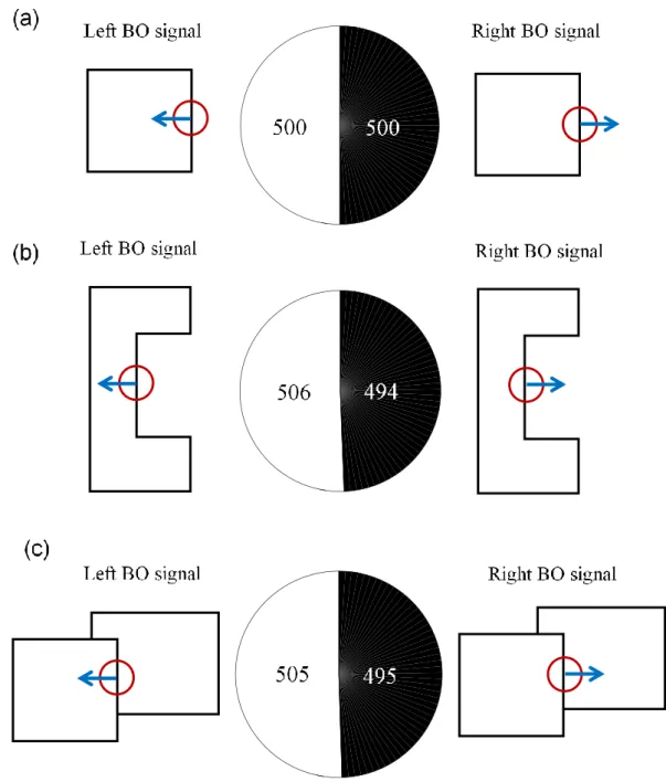
Model outputs were categorized according to the direction of the BO signal located at the position of the neuron’s receptive field, represented by the red circle in Figure 4.1. The neuron responds selectively to an object placed on the left of its receptive field. This coincides with a left BO signal. The model outputs left-facing vectors at chance-level for all three stimuli.

Although this method of assigning initial vectors fails to reproduce the data from physiological experiments at a significant rate, it is interesting to note that surfaces coinciding with various depth order perception was reproduced. For example, Figure 4.2

𝑬(𝑥, 𝑦, 0) = ( 𝜕 𝜕𝑥𝐵(𝑥, 𝑦) 𝜕 𝜕𝑦𝐵(𝑥, 𝑦)) ≈1 2( 𝐵(𝑥 + 1, y) − 𝐵(𝑥 − 1, y) 𝐵(𝑥, y + 1) − 𝐵(𝑥, y − 1)). (4.1)

(39)

and Figure 4.3 shows the two types of surfaces, an object or a hole, reproduced by the model. In addition, for an occluding square, a left (or right) BO signal at the location of the neuron’s receptive field coincides with three different depth order percepts, respectively (Figure 4.4 or Figure 4.5).

(40)

Figure 4.1 Categorization of calculated BO signals from randomly assigned initial vectors.

The red circle represents a neuron’s receptive field located at the border of (a) a square, (b) a C-shaped figure and (c) an overlapping square. These figures are similar to those used in physiological experiments outlined in Figure 1.4. Assigning initial vectors randomly (1000 combinations) results in BO signals in the left or right direction at chance-level. Random initial vectors cannot reproduce physiological data consistently.

(41)

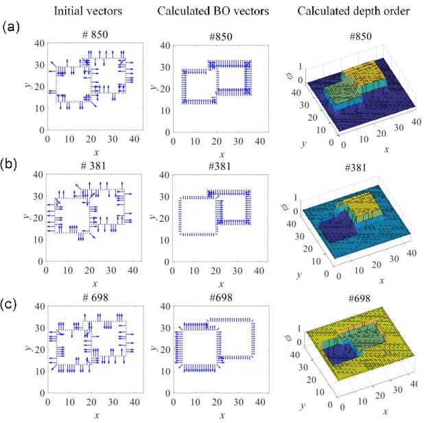
Figure 4.2 Calculated BO vectors and depth order for a square with randomly assigned initial vectors.

Example of the different percepts categorized as (a) a left BO signal and (b) a right BO signal in Figure 4.1a. A left BO signal coincides with the percept of a square object, whereas a right BO signal coincides with a square hole. The element number in the set of 1000 randomly assigned initial vectors is shown above the respective results.

(42)

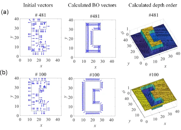
Figure 4.3 Calculated BO vectors and depth order for a C-shaped figure with randomly assigned initial vectors.

Example of the different percepts categorized as (a) a left BO signal and (b) a right BO signal in Figure 4.1b. A left BO signal coincides with the percept of a C-shaped object, whereas a right BO signal coincides with a C-shaped hole. The element number in the set of 1000 randomly assigned initial vectors is shown above the respective results.

(43)

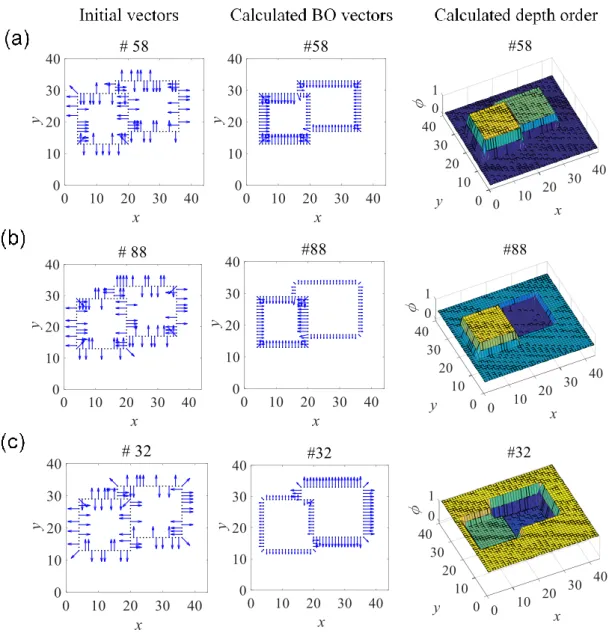
Figure 4.4 Calculated BO vectors and depth order for an overlapping square with randomly assigned initial vectors.

Example of the different percepts categorized as a left BO signal in Figure 4.1c. Unlike the square and C-shaped figure, a left BO signal coincides with three distinct depth order percepts (a~c). The element number in the set of 1000 randomly assigned initial vectors is shown above the respective results.

(44)

Figure 4.5 Calculated BO vectors and depth order for an overlapping square with randomly assigned initial vectors.

Example of the different percepts categorized as a right BO signal in Figure 4.1c. Unlike the square and C-shaped figure, a left BO signal coincides with three distinct depth order percepts (a~c). The element number in the set of 1000 randomly assigned initial vectors is shown above the respective results.

(45)

4.2 Determining suitable initial vectors

To reproduce the data from physiological experiments, suitable initial vectors must be assigned. There are two types of junctions that might serve as useful cues: (a) L-junction and (b) T-junctions.

First, let us consider L-junctions. The contour of an occluding object is essentially a simple closed curve. For a closed curve 𝐶(𝑠) described by its arc length 𝑠, the total curvature along the curve is a positive value ∫ 𝜅(𝑠)𝑑𝑠_𝑠 > 0. In simple terms, there are more acute angles than obtuse angles in the contour of an occluding object. This is demonstrated in Figure 4.6 for the three figures used. Vectors facing the inner-side of the L-junctions might serve as suitable initial values. Physiological experiments reveal that some neurons in area V2 respond selectively to bent lines, especially to acute-angled lines, placed in their receptive fields [26], [27]. Gestalt psychologists observed that the convex side of curves are likely to be perceived as the inner-side of an object [28].

Next, consider T-junctions. There are several possible depth-order combinations at around the junction, as illustrated in Figure 4.7. Initial BO vectors facing the surface with the largest depth order value. Since there are several possible BO signals, T-junctions may not be a reliable cue for the determination of initial vectors. In summary, initial vectors were assigned facing the inner side of L-junctions using Eq. (4.1), whereas zero vectors were assigned at straight-line segments and T-junctions for the three figures.

Simulations were conducted for 𝑡 = 10000 to confirm the suitability of these initial vectors. The time course from 𝑡 = 0 to 𝑡 = 10000 of 𝑬(𝑥, 𝑦, 𝑡) and 𝜙(𝑥, 𝑦, 𝑡) is shown for the three stimuli (Figure 4.8, Figure 4.9 and Figure 4.10). he red circle represents the approximate location of the receptive field for the neuron examined in the physiological experiment by Zhou et al. (2000). The neuron responds selectively to an

(46)

object on the left side of its receptive field. BO signals (vectors) located in the red circle point towards the left, qualitatively matching experimental results. Vectors around the concave region of the C-shaped figure were corrected to face the occluding object, and not the background. After sufficient updating of vectors reflect, relative depth order for all three stimuli how they are actually perceived. Notably, the occluding rectangle has a larger 𝜙 value than the occluded rectangle and vector magnitudes are adjusted automatically to reflect this.

These results show that setting initial vectors facing the acute side of L-junctions is an appropriate method to reproduce the left object-side selectivity of the neuron used in physiological experiments. The next subsection will compare the response of the V2 neuron with model outputs.

(47)

Figure 4.6 The contour of an occluding object has more acute angles than obtuse angles.

Calculated depth order and BO signals which coincide with perception of (a) a square, (b) a C-shaped figure and (c) an overlapping square. For all three examples, the BO signal in the red circle (receptive field) point in the left direction. This agrees qualitatively with the response of the neuron in Figure 1.4. The outline of an occluding figure is a simple closed curve. This means that there are more acute angles (blue) than obtuse angles (yellow). Acute angles might be a reliable cue to reproduce data from physiological experiments.

(48)

Figure 4.7 Several possibilities for initial vectors exist at T-junctions.

Examples of possible initial vectors at the T-junction in the figure of (a) an overlapping square. The T-junction at the red square is examined. Numbers in the brackets represent the depth order value of the surface. The blue arrow points towards the surface with the highest depth order value. Initial vectors (blue arrows) coinciding with the three respective percepts in (b) Figure 4.4 and (c) Figure 4.5.

(49)

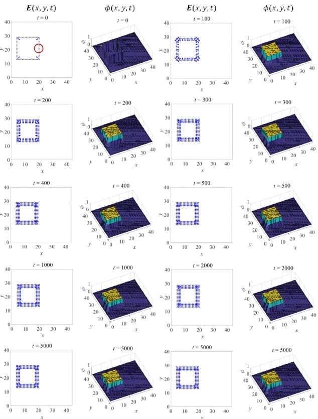
Figure 4.8 Time course of vector field and scalar field for a square.

Evolution of 𝑬(𝑥, 𝑦, 𝑡) and 𝜙(𝑥, 𝑦, 𝑡) over time 𝑡 = 0~10000 for a square. The red circle represents the location of the receptive field.

(50)

Figure 4.9 Time course of vector field and scalar field for a C-shaped figure.

Evolution of 𝑬(𝑥, 𝑦, 𝑡) and 𝜙(𝑥, 𝑦, 𝑡) over time 𝑡 = 0~10000 for a C-shaped figure. The red circle represents the location of the receptive field.

(51)

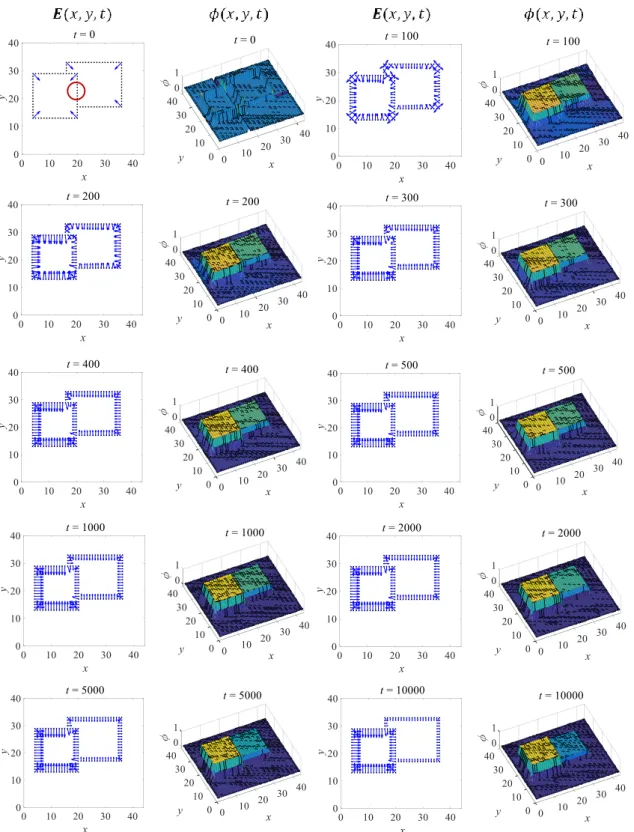
Figure 4.10 Time course of vector field and scalar field for an overlapping square.

Evolution of 𝑬(𝑥, 𝑦, 𝑡) and 𝜙(𝑥, 𝑦, 𝑡) over time 𝑡 = 0~10000 for an overlapping square. The red circle represents the location of the receptive field.

(52)

4.3 Reproduction of experimental findings

4.3.1 Modeling V2 neuron responses

The relationship between BO signals and responses of object-side selective neurons in V2 must be modeled to make a direct comparison between model results and neuronal responses. The response of a neuron with right object-side (left object-side) selectivity is termed as V2_right (V2_left). Outputs of these neurons can be modeled as the sum of the neuron’s response to a border in its receptive field and ownership information,

Therein, Border is positive when a border is located in the neuron’s receptive field; Owner_right and Owner_left are either positive or zero. Based on the model proposed above, a BO signal in the horizontal direction 𝐸_𝑥 can be defined as the difference in outputs of pairs of neurons with object-side selectivity in opposite directions,

In Figure 4.11, a vertical edge is located in the receptive field, invoking a positive Border response. An object is located to the left of the receptive field. Ownership information pertaining to an object on the left is thus a positive value (Owner_left > 0), whereas ownership information pertaining to an object on the right is zero (Owner_right = 0). The resulting BO signal in the horizontal direction is negative, 𝐸_𝑥 = −Owner_left < 0, indicating the existence of an object on the left. The same approach is taken to calculate BO signals in the vertical direction 𝐸_𝑦.

Model outputs were found to qualitatively match the relative magnitude of neuron responses to the three stimuli up to 𝑡 = 2000; neuron responses are largest for the square and smallest for the C-shaped object. The absolute value of the 𝒙̂ component at the center

V2_right = Border+Owner_right, (4.2)

V2_left = Border + Owner_left. (4.3)

(53)

of the red circle |𝐸𝒙(20,21,2000)| was used to qualitatively compare model responses with physiological data. Notably, for the overlapping rectangle in Figure 4.12, vectors were scaled to a magnitude of 2 to account for the existence of two objects of different depth order. |𝐸_𝒙(20,21,2000)| for the three figures are 0.92, 0.78 and 0.89, respectively.

Figure 4.13 shows relative model response and neuronal response for the three stimuli.

Values for relative model response were scaled to a maximum of 1, based on the model response to the square. Model responses for the C-shape and the overlapping square are lower than that for the square. This matches V2 neuronal responses for similar stimuli used in Zhou et al. (2000). The proposed model captures the qualitative nature of the response of the neuron towards the three benchmark stimuli better than previous models [17], [18], [21]. The method of recording neuron responses is a possible explanation why physiological data and model outputs qualitatively match. Responses of neurons were only recorded for the first 200 ms after stimulus onset. Neuron recordings for more than 200 ms might present a different property. Craft et al. (2007) also specify a time frame for their model output.

Note that in theory, vector magnitude should be of equal value after updating. Figure

4.14 shows relative model responses after 500, 1000, 2000, and 10000 iterations. Relative

model response qualitatively match physiological data for the first 2000 iterations. Model responses at 10000 iterations show that the model does not update vectors for a C-shaped figure after a certain threshold of iterations. This might be due to the initial vectors facing outwards at the concave region. The relative response to the occluded figure exceeds the relative response to the square at 10000 iterations. Observations were made that the cause of this is due to the magnitude of occluded-object vectors decreasing as time progresses (Figure 4.10).

(54)

Figure 4.11 Data adapted from Zhou et al. (2000) is used to illustrate how to compare BO signals with V2 neuron responses.

A horizontal BO signal 𝐸_𝑥 can be obtained from the difference in response of a pair of V2 neurons with opposite object-side selectivity (V2_left ≃ 50 and V2_right ≃ 19). Neuron receptive fields are represented by circles, whereas arrows represent the neurons’ object-side selectivity and response strength. The difference in response of these neurons is a negative BO signal in the horizontal direction 𝐸_𝑥 = V2_right− V2_left ≃ −31 , signifying an object to the left of the receptive field.

(55)

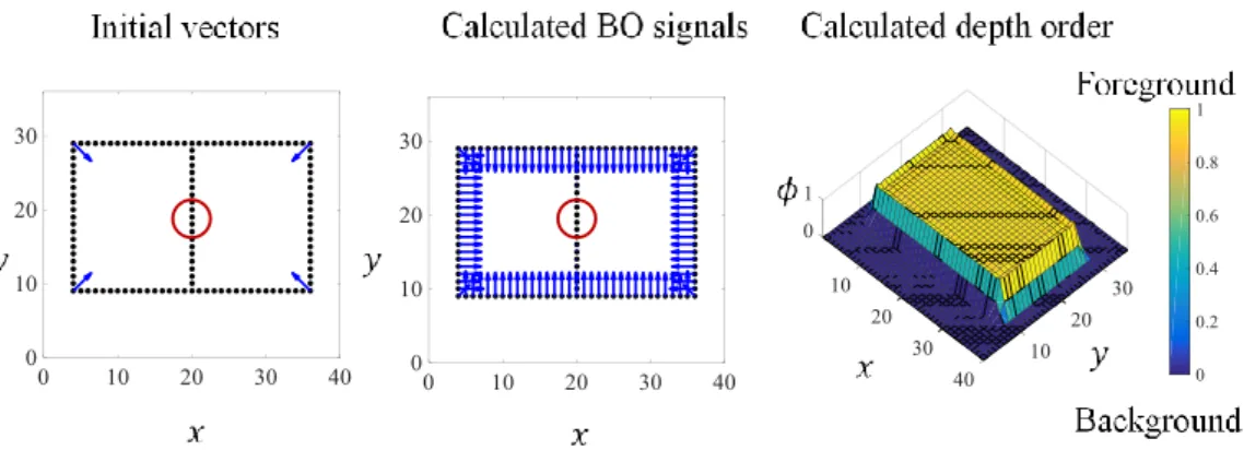
Figure 4.12 Initial vectors, calculated BO signals and depth order for figures similar to the stimuli used in physiological experiments for a V2 neuron with selectivity for an object to the left of its receptive field.

Respective depth order scalar field agrees with the perception of (a) a square, (b) a C-shape, and (c) an overlapping square. Red circles indicate the approximate location of the neuron’s receptive field in respect to the figure. Calculated BO signals face to the left, agreeing qualitatively with the neuron’s object-side selectivity. The absolute value for 𝒙

̂ component at the center of the red circle, |𝐸_𝑥(20,21,2000)|, is displayed on the respective figures (a. 0.92; b. 0.78; c. 0.89).

(56)

Figure 4.13 BO signals calculated from experimental data produced by Zhou et al. (2000) and relative model response from the proposed model in comparison with existing models.

Neuronal responses are shown for three benchmark stimuli (a C-shaped figure, an occluded figure, and a square). Responses to the stimuli are arranged in ascending order of response strength. Proposed model responses are based on absolute values for 𝒙

̂ component at the center of the red circle, |𝐸_𝑥(20,21,2000)|, in Figure 4.12. The red circle in the respective figures represent the neuron’s receptive field, and the arrow represents the direction of the BO signal. The proposed model qualitatively reproduces the difference in response of the neuron to the three stimuli for 𝑡 = 2000. In comparison, existing models are incapable of reproducing this phenomenon [17], [18], [21].

(57)

Figure 4.14 BO signals calculated from experimental data produced by Zhou et al. (2000) and relative model response for 500, 1000, 2000, and 10000 iterations.

In general, relative model responses converge to 1 as the number of iterations increase. However, the response of the model to the C-shaped figure ceases to increase, and the relative response to the occluded figure exceeds the relative response to the square (10000 iterations).

(58)

4.3.2 Transparent overlay

Some neurons in V2 which possess object-side selectivity also respond selectively to “transparent” occluding objects [29]. For example, the image in Figure 4.15b can be perceived as either a light-grey rectangle overlapping a grey rectangle, or a dark-grey rectangle overlapping a light-dark-grey rectangle. Both rectangles are perceived to be “transparent”. Consider a neuron with a receptive field represented by the red circle, located at a vertical border. An occluding object is located on the left of the receptive field. This agrees with perception. Figure 4.15a is perceived as an opaque light-grey rectangle overlapping an opaque dark-grey rectangle. Similar to Figure 4.15b, the occluding object is located on the left-side of the receptive field. In contrast, the occluding object is located on the right-side of the receptive field in Figure 4.15c. This is because the image is perceived as four separate squares. The pattern and luminance in all three examples are the same. These three figures are similar to those used in physiological experiments by Qiu and von der Heydt (2007) [29].

Calculated BO signals after 𝑡 = 1000 iterations and the enlarged region around (20,17) is shown for the three figures in Figure 4.15. The direction of the circled vectors in the enlarged region for Figure 4.15a and Figure 4.15b point to the left. In contrast, the direction of the circled vector in Figure 4.15c faces the right. The modulation (direction) of these vectors agree with BO signals from actual physiological experiments by Qiu and von der Heydt (2007) [29]. The model is capable of qualitatively reproducing BO signals despite the absence of luminance information as an input.

(59)

Figure 4.15 BO signals calculated for borders of (a) overlapping opaque rectangles, (b) overlapping transparent rectangle, and (c) four separated squares.

Only borders, void of luminance information, was used as model inputs. The direction of vectors at (20,17) agree with BO signal modulation for a neuron with a receptive field represented by the red circles on the images [29].

(60)

4.3.3 Zero BO signal

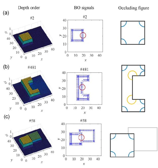
Physiological experiments have demonstrated that for specific figures, the BO signal at a border between two objects can take a value of zero [30]. Figure 4.16 shows a figure where the occluding object and the occluded object is unclear. The image can be perceived as two rectangles placed side-to-side. This figure is similar to the one used in the physiological experiment. Calculated BO signals (vectors) at the red circle, which represents the location of a receptive field, are zero. This agrees qualitatively with experimental data. Depth order for both objects are the same despite the existence of a border.

(61)

Figure 4.16 BO signals and depth order for a figure with a zero BO signal at the border.

Zero vectors are assigned along the central border. The regions on both sides have equally valued depth order. The neuron used in physiological experiments shares the same location for the receptive field represented by the red circle [30]. BO signals from experiments were found to be zero, as well.

(62)

4.4 Complex patterns

Several complex patterns which do not have corresponding data from physiological experiments were also tested to examine the robustness of the model towards shape and occlusion (Figure 4.17). These include (a) a complex Y-shaped figure, (b) an O-shaped figure, (c) C-shaped figure occluding a square, (d) interlocking L-shapes and (e) four overlapping cards. The evolution of 𝑬(𝑥, 𝑦, 𝑡) and 𝜙(𝑥, 𝑦, 𝑡) over time for the respective figures are shown in Figure 4.18 to Figure 4.22.

Figure 4.17a shows a figure with several concave regions. Initial vectors point towards these concave regions in Figure 4.18. As time progresses, these vectors are corrected to point to the object. However, the model is incapable of reproducing the perception of an O-shaped given the initial vectors set to face the acute side of the L-junctions at the perimeter of the hole (Figure 4.19). Figure 4.17b shows a figure with both local concavity and occlusion. The model is capable of correcting vectors facing the locally concave region and resolve depth order for the two objects simultaneously (Figure 4.20). Figure 4.17d shows an image perceivable as two interlocking L-shapes. Figure 4.17e is a similar figure. It can be perceived as four overlapping cards. As iteration 𝑡 increases, calculated depth order converges at a flat surface; the depth order of the two (or four) objects carries the same value. However, it is interesting to note that at 𝑡 = 100, depth order resembles perception.

(63)

Figure 4.17 Five figures with problems of shape, occlusion, or both.

Simulations were conducted for (a) a complex Y-shaped figure, (b) an O-shaped figure, (c) a C-shaped figure occluding a square, (d) interlocking L-shapes and (e) four overlapping cards.

(64)

Figure 4.18 Evolution of BO signals and depth order over time for a figure perceivable as a Y-shaped object.

(65)

Figure 4.19 Evolution of BO signals and depth order over time for a figure perceivable as an O-shape.

Evolution of 𝑬(𝑥, 𝑦, 𝑡) and 𝜙(𝑥, 𝑦, 𝑡) over time 𝑡 = 0~2000. Model outputs do not agree with the perception of an O-shaped figure.

(66)

Figure 4.20 Evolution of BO signals and depth order over time for a figure perceivable as a C-shape occluding a square.

(67)

Figure 4.21 Evolution of BO signals and depth order over time for a figure perceivable as a interlocking L-shapes.

(68)

Figure 4.22 Evolution of BO signals and depth order over time for a figure perceivable as overlapping cards.

(69)

4.5 Evaluation of results

Simulation results demonstrate that the model was capable of assigning BO correctly for figures with occlusion without the use of a specific junction detector. Although a T-junctions may serve as an important occlusion cue in some cases, there are also situations where T-junctions are not formed by an intersection of three surfaces of differing depth order. Figure 4.23 shows four ways in which a local T-junction can be interpreted as. For all four cases, the rotation at the T-junction is zero. In particular, the depth order in Figure

4.23c-d can be seen at T-junctions in figures containing ambiguous borders (Figure 4.16).

The proposed model uses global contextual information to determine a unique solution for various perceptual problems involving depth order.

The proposed model simultaneously produced BO signals and depth order that match perception. Simulation results demonstrate that the model is highly dependent on initial vectors. To reproduce data from physiological experiments, initial vectors were provided in a deterministic manner through L-junction detectors. Spatial propagation of contextual information using the update rule automatically determines BO signals regardless of local concavity. Calculating curvature might serve as a replacement to L-junction detectors. This would allow simulations of figures with more complex shapes to be carried out.

Although initial vectors based on L-junctions alone are useful, they are insufficient to reproduce depth order perception for figures such as an O-shaped figure. Reversing the vectors at the center, as shown in Figure 4.24 demonstrates the importance of initial vectors. A more global method of initial vector determination is required to reproduce human perception.

(70)

Figure 4.23 Image of a T-junction, four possible perceptions of depth order and their corresponding BO signals.

Numbers on the surfaces represent depth order values. Short vectors are of length one, while long vectors are of length two. (a) and (b) are T-junctions where the surface to the top of the T-junction has the highest depth order value of the three. However, adjoined surfaces of equal depth order value, such as in (c) and (d) may also form T-junctions. Notably, the local curl at the cross-mark for all four examples is zero.

(71)

Figure 4.24 Reversing initial vectors at the inner border produces depth order consistent with perception of an O-shaped figure.

L-junctions are vital cues to occluded object perception, but are insufficient to reproduce the perception of an O-shaped figure. For example, reversing initial vectors around the border perceived as the hole reproduces this percept.

(72)

5 Deductions and model comparisons

5.1 Mathematical foundation for present models

5.1.1 Spatial distribution of intra-cortical connections in the model by Li

Deductions can be made about the spatial distribution of intra-cortical connections from the update rule in Eq. (3.4). For example, the 𝒙̂ component of the update rule

𝜕

𝜕𝑡𝐸𝑥(𝑥, 𝑦, 𝑡) reveals neural connections for a neuron at (𝑥, 𝑦) with either a right object-side (𝐸_𝑥(𝑥, 𝑦, 𝑡) > 0), or a left object-side ((𝐸_𝑥(𝑥, 𝑦, 𝑡) < 0) selectivity. A closer look at the right hand side of this update rule shows that this neuron at (𝑥, 𝑦) has connections to other neurons with either left or right object-side selectivity 𝜕

2

𝜕𝑦2𝐸𝑥(𝑥, 𝑦, 𝑡) and neurons either up or down object-side selectivity − 𝜕2

𝜕𝑥𝜕𝑦𝐸𝑦(𝑥, 𝑦, 𝑡). The differentiation operators dictate the spatial distribution of these connections. Figure 5.1 illustrates possible intra-cortical connection for a neuron with a right object-side selectivity, with a receptive field represented by a red oval on the image. As seen in Figure 5.1a, connections with left or right object-side selective neurons 𝐸_𝑥 is equivalent to diffusion in the horizontal 𝑦 -direction. Figure 5.1b, illustrates connections with left or right object-side selective neurons 𝐸_𝑦 positioned diagonally.

The structure of these connections is similar to that of the model by Li (2000). A method to qualitatively compare the two is proposed. Spatial filters for 𝐸_𝑥 and 𝐸_𝑦 in

Eq. (3.8) can be expressed as weights 𝑤_𝑥(𝑥, 𝑦) ≝ 𝜕2

𝜕𝑦2𝐺𝜎(−𝑥−, 𝑦) and 𝑤𝑦(𝑥, 𝑦) ≝ −𝜕2

𝜕𝑥𝑦𝐺𝜎(−𝑥, −𝑦). Discrete weights for a neuron positioned at (0,0) with a left or right object side selectivity can thus be expressed as

(73)

Weights can then be expressed as vectors 𝒘 = (𝑤𝑥, 𝑤𝑦)T of magnitude ‖𝒘‖ = √𝑤𝑥2+ 𝑤𝑦2. Weights for 𝐸𝑥(𝑥, 𝑦, 𝑡) are visualized in Figure 5.2a using weights consisting of Gaussian derivative kernels with standard deviation 𝜎 = 1. Each vector illustrates the direction of 𝒘, whereas pixel intensity represents vector magnitude ‖𝒘‖. Vector magnitudes were normalized to 1.

Horizontal connections proposed by Li (2000) were visualized in a similar manner using weights for a right object-side selective neurons. In particular, the weights which describe connections to four types of other object-side selective neurons were used (left, right, up, down). These weights are visualized in Figure 5.2b. The nature of deduced intra-cortical connections from the proposed model and those from the model by Li (2000) were found to be qualitatively similar. However, the results cannot be treated as ground truths since the nature of horizontal connections in area V2 are currently unknown.

𝜕 𝜕𝑡𝐸𝑥(0,0, 𝑡) = ∑ ∑ 𝑤𝑥(𝑖, 𝑗)𝐸𝑥(𝑖, 𝑗, 𝑡) 𝑗 + ∑ ∑ 𝑤_𝑦(𝑖, 𝑗)𝐸_𝑦(𝑖, 𝑗, 𝑡). 𝑗 𝑖 𝑖 (5.1)

(74)

Figure 5.1 Plausible neural network for a neuron that responds selectively to a vertical border and an object to the right of its receptive field.

Neuron receptive fields are represented by ovals; arrows represent their object-side selectivity. The neuron focused on has a red oval as a receptive field. Black circles in area V2 represent neurons with receptive fields on the image. Neurons are either connected by excitatory or inhibitive neural connections, according to their relative location and object-side selectivity. Connections with (a) right (or left) object object-side selective neurons were derived from the 𝐸_𝑥 component; (b) up (or down) object side selective neurons were derived from the 𝐸𝑦 component in in Eq. (3.4).

(75)

Figure 5.2 Charactertistics of neural weights 𝒘 for a neuron at spatial position (𝟎, 𝟎) with a right object-side selectivity, visualized using vectors.

Vector magnitudes ‖𝒘‖are represented by pixel intensity. The characteristics of neural weights for (a) the proposed model are qualitatively similar to those of (b) the model by Li (2000).