渦糸の伸縮
-
局所誘導方程式の初期値問題としてー
日大・理工 紺野 公明 (Kimiaki Konno)’
富山大・工角畠 浩 (Hiroshi Kakuhata)**
’Department of Physics, College of Science and Technology,
Nihon University, **Toyama University
1
初めに
我々は三次元空間で伸縮する弦 (string, fflament) の運動について研究を行っ ている.$[1][2][3]$ この報告では局所誘導方程式 (渦糸の運動方程式) $r_{t}=r_{s}\cross r_{ss}$ (1) について渦糸の伸縮と言う立場から初期値問題を考える. ここで, $r$ は位置 ベクトル $r=(X, \mathrm{Y}, Z)$, (2) を表す. 方程式の厳密解は接線ベクトノt $=\partial r/\partial s$ の絶対値が $|t|=1$ を満たすた め伸縮がない. では初期値として局所的に伸縮を持つ渦糸を考え, (1) の方程 式に従って時間発展させたら, 伸縮のある領域とその渦糸の形が時間経過と 共にどの様な運動を行うのか興味があり数値計算を行う. 初期値として, [1] 渦糸ソリトンとそれを基に作られた伸縮を持っ波形,
[2] 2次元$j\triangleright ―$y状の形 状で伸縮を持つ波形, それと [3] 2次元の孤立波の形状で伸縮のある波形の三 種類を考える. 波形の伸縮性を理解するため例としてシェアー流の中での渦糸の運動に ついて数値計算を行う. そのシェアー流によって渦糸が変形され, それを定 義された局所伸縮という言葉で表す$\ovalbox{\tt\small REJECT}$ 次の章では渦糸の局所伸縮の定義を行う. 第3章ではシェアー流の中での 渦糸の運動を調べる. 第 4 章では与えられた初期値について数値計算の結果 を示す. 最後にまとめを行う.2
伸縮の定義
局所的な渦糸の長さ市(s)
は 市 $=\sqrt{(\mathrm{d}X)^{2}+(\mathrm{d}\mathrm{Y})^{2}+(\mathrm{d}Z)^{2}}$ (3) で与えられ, (1) 式の弧長 $s$ で書き直す. $\mathrm{d}l(s)=\sqrt{(X_{s})^{2}+(\mathrm{Y}_{s})^{2}+(Z_{s})^{2}}\mathrm{d}s$ (4) 数理解析研究所講究録 1311 巻 2003 年 155-167155
局所的な渦糸の伸縮 $l_{s}$ を次のように定義する. $l_{s}= \frac{\mathrm{d}l}{\mathrm{d}s}=\sqrt{(X_{\epsilon})^{2}+(\mathrm{Y}_{\epsilon})^{2}+(Z_{s})^{2}}$
.
(5) $l_{\epsilon}=1$ は伸ひのないことを意味し, $l_{\epsilon}>1$ は渦糸が伸ひていることを, $l_{s}<1$ は渦糸が縮んでいることを表す.3
シェアー流と渦糸の伸ひ
渦糸の伸縮を見るために $x$ 方向に作用するシェアー流の中での渦糸の運動を 見る. 運動方程式を -Y$r_{t}=r_{\epsilon}\cross \mathrm{r}_{\epsilon\epsilon}+\alpha\tanh\div \mathrm{e}_{1}$
.
(6)$\Delta$
で与える. $e_{1}$ は $x$ 方向の単位ベクトルである. 定数を $\alpha=2$ と $\Delta=1$ に
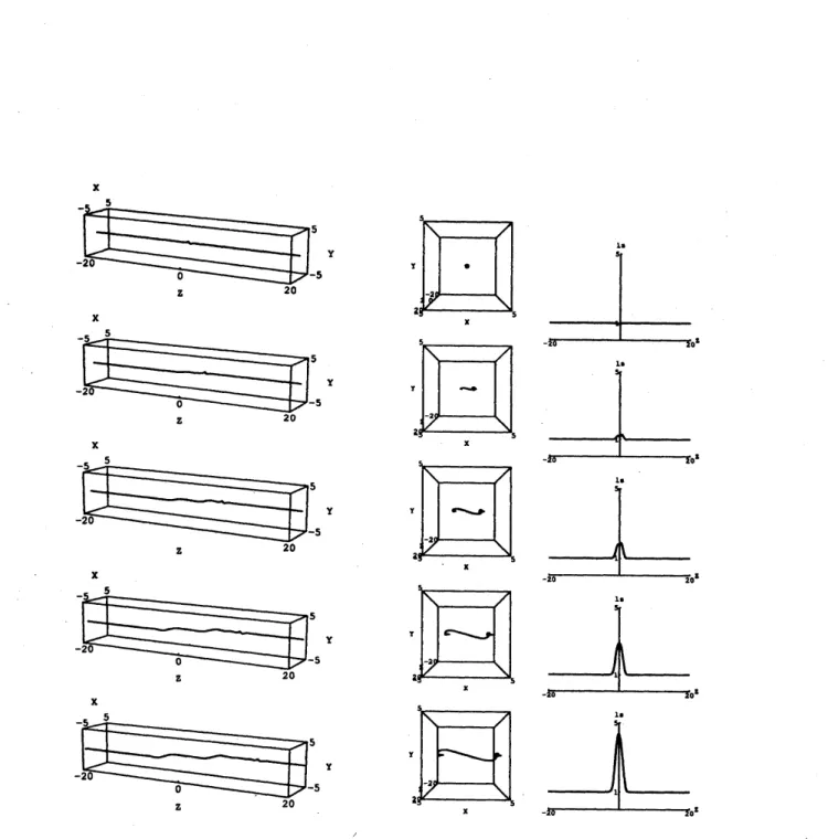
取る. 初期値として渦糸ソリトン解 $X= \frac{\lambda_{I}}{\lambda_{R}^{2}+\lambda_{I}^{2}}\sin(2\Omega+\delta)\mathrm{s}\mathrm{e}\mathrm{c}\mathrm{h}(2\Theta+\epsilon)$, $\mathrm{Y}=-\frac{\lambda_{I}}{\lambda_{R}^{2}+\lambda_{I}^{2}}\cos(2\Omega+\delta)\mathrm{s}\mathrm{e}\mathrm{c}\mathrm{h}(2\Theta+\epsilon)$, (7) $Z=s- \frac{\lambda_{I}}{\lambda_{R}^{2}+\lambda_{I}^{2}}\tanh(2\Theta+\epsilon)$ を考える. $\Omega,$ $\Theta$ 及ひ定数は $\Omega=\lambda_{R}s-\omega_{R}t$, $\Theta=\lambda_{I}s-\omega_{I}t$, $\tan\delta=-\frac{2\lambda_{R}\lambda_{I}}{\lambda_{R}^{2}-\lambda_{I}^{2}}$, $\epsilon=-\frac{1}{2}\log\frac{|c_{0}|^{2}}{4\lambda_{I}^{2}}$ (8) で与えられる. $c_{0}$ は定数である. 波数 $\lambda=\lambda_{R}+\mathrm{i}\lambda_{I}$ と振動数 $\omega=\omega_{R}+\mathrm{i}\omega_{I}$ との関係は次の分散式から決められる. $\omega=2\lambda^{2}$ (9) 数値計算の結果を図 1 に示す. 左図は初期に与えた渦糸ソリトンは正の方 向に伝搬しているが, シェアー流のため渦糸の一部が時間と共に引き延ばさ れている波形を示している. $z$ 軸の正の方向から見た中央の図で渦糸が $x$ 方 向の正と負の両側の方向に引き延ばされていく様子を見ることができる. 右 図は局所伸縮を表すために横軸を $Z$ に縦軸を局所伸縮 $l_{s}$ に取ってある. 伸 ばされている位置とその大きさを図から読みとることが出来る.
156
4
初期値問題
4.1
渦糸ソリトン 先す, 初期値として渦糸ソリトン解 (7) に伸縮を与える因子 $A$ を掛けた次の 式を考える. $X=A \frac{\lambda_{I}}{\lambda_{R}^{2}+\lambda_{I}^{2}}\sin(2\Omega+\delta)\mathrm{s}\mathrm{e}\mathrm{c}\mathrm{h}(2\Theta+\epsilon)$, $\mathrm{Y}=-A\frac{\lambda_{I}}{\lambda_{R}^{2}+}$\lambdaI2.coe(2\Omega+\mbox{\boldmath$\delta$})ae
出
(2\ominus+\epsilon),
(10) $Z=s- \frac{\lambda_{I}}{\lambda_{R}^{2}+\lambda_{I}^{2}}\tanh(2\Theta+\epsilon)$, ここで, $A=1$ とすると方程式(1) の厳密解を与え局所伸縮を持たない. 局所伸縮は $l_{\epsilon}^{2}=A^{2}(X_{\epsilon}^{2}+\mathrm{Y}_{\epsilon}^{2})+Z_{s}^{2}$ $=1+ \frac{4\lambda_{I}^{2}}{\lambda_{R}+\lambda_{I}^{2}}(A^{2}-1)[\mathrm{s}\mathrm{e}\ ^{2}(2 \Theta+\epsilon)-\frac{\lambda_{I}^{2}}{\lambda_{R}^{2}+\lambda_{I}^{2}}\mathrm{s}\mathrm{e}\mathrm{c}\mathrm{h}^{4}(2\Theta+\epsilon)]$ (11) で与えられる. $A<1$ のとき局所的に縮んだ領域を持ち, $A>1$ のとき局所 的に伸ひた領域を持つ. 数値計算は, $\lambda=1.5+\mathrm{i}$, へ $=1$ とし $A$ の値 1,08
と 12 の場合につい て行いそれぞれ図 2, 図3 及ひ図 4 に示してある. 特徴的なことは伸縮性を持 つ初期値についてはその伸縮のある領域が時間経過にも関わらず同じ領域に 固定されているいるように見える. 波形の運動については, 縮のある波形は 速く伝搬し, 次に伸縮のない波形, 一番遅いのが伸ひのある波形であることが 観測された.4.2
2
次元ループ形状を持つ初期値
初期値として2
次元ループ形状の波形 $X=0$, $\mathrm{Y}=A$sech$ks$, (12) $Z=s-2\tanh ks$ を考える. 局所伸縮は $l_{\epsilon}^{2}=1+4(A^{2}-1)\mathrm{s}\mathrm{e}\ ^{2}ks\tanh 2ks$.
(13)157
で与えられる. ただし, $k=2$ に取ってある. $A$ として局所伸縮のない場合, 縮んでいる場合と伸びている場合に対応す る 1,
08
と 12 のそれぞれの値に対し図 5, 図6
と図7
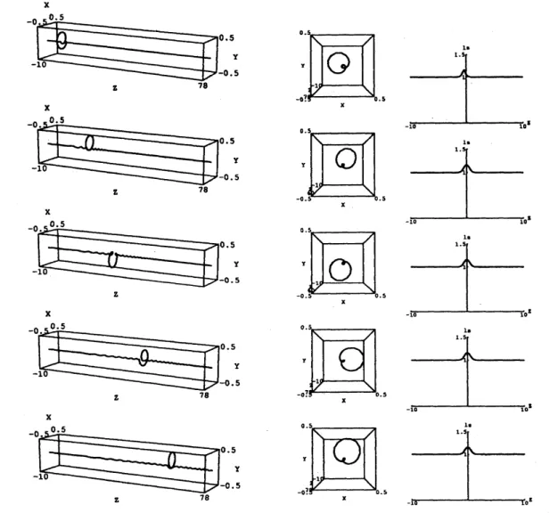
に結果を示した. この 場合も渦糸ソリトンと同様, 伸縮のある領域は時間経過をしても初期で与え られた領域に固定されたままであった. より詳しくは伸びのあるときは伸縮 のある領域が初期で与えあれた領域の周りを時間経過によって前後運動して いた. この初期値で特徴的なことは伸びがない $A=1$ ときはループ状の波形 は正の方向に伝搬するが, 伸ひ $A=1.2$ と縮み $A=0.8$ を持つ波形はその伸 縮している領域にピンニングされ, 計算時間内では伝搬していないことが観 測された.4.3
2
次元孤立波形状を持つ初期値
2 次元孤立波形状を持つ初期値 $X=0$, $\mathrm{Y}=A$sech$ks$, (14) $Z=s$ を考える. 局所伸縮は$l_{\mathit{8}}^{2}=1+k^{2}A^{2}$
sech2
$ks\tanh 2ks$.
(15)で与えられる. ここで $A=1$ と $k=2$ にとり数計算を行った結果を図
8
に示 す. 伸ひのある場所はやはり初期に与えた場所に固定されているが振幅は小 さくなると共に正と負の方向に伝搬する回転する波を放出していることが見 られた.5
終わりに
我々は局所伸縮の定義を与えた. 局所誘導方程式に局所伸縮を持つ初期値を 与え, その伸縮が時間経過と共にどのように変わる力\searrow
また, 波形が期間経過 と共にどのように変化していくかを数値的に調べた. その主な結果は次の2
点である. (1) 初期値で与えた伸縮のある領域は時間が経過してもほぼ同じ領域にフ リーズされていた. (2) (12) で与えた初期に伸縮を持つ波形は, 時間経過後もその伸縮のある領 域に波形がピンニングされていた.158
これらの局所伸縮のフリージング現象と波形のピンニング現象の詳細な 解析はこれからの課題である. 実験的にはタンク内に作られる渦糸には軸方 向の流れが生成されるのでその効果を取り入れなければならない. その軸方 向流を持つ流れの中での局所伸縮のフリージング現象とか波形のピンニング 現象がどの様になるのか興味がある. 伸ひ縮の具体的例として局所誘導方程式にシェアー流を加え渦糸ソリト ンの時間発展を見た. よく知られたシェアー流の効果で渦糸が伸びていく過 程が見られた. しかし, 局所伸縮の定義を与え, その立場で渦糸の伸ひ縮みを 表現したの初めてであると思う.
References
[1] Kimiaki Konno and Hiroshi Kakuhata, An integrable system with two
hierarchies and related topics in ”$\mathrm{N}\mathrm{o}\mathrm{n}\mathrm{l}\mathrm{i}\mathrm{n}\mathrm{e}\mathrm{a}\mathrm{r}\mathrm{P}\mathrm{h}\mathrm{y}\mathrm{s}\mathrm{i}\mathrm{o}\mathrm{e}$:Theory and
Exper-iments $\mathrm{I}\mathrm{I}^{n}$ (World Scientific) to appear in (2003).
[2] K. Konno and H. Kakuhata, Stretching and shrinking of loop soliton
interacting with external field presented in
NEEDS
2002, Cadiz, SpainJune,
2002.
[3] K. Konno and H. Kakuhata, Stability of string soliton by balancing
between its stretching and shrinh.ng, to be submitted for publication.
$\mathrm{x}$
$\mathrm{x}$
Figure 1: Time evolution offilament(left), its top view ffom the positive $Z$
axis(middle) and local stretch 1, $\mathrm{v}\mathrm{s}$
.
$Z$ (right) at$t=0,0.5,1,1.5,2$
ffomthe top to the bottom.
$\mathrm{x}$
$\mathrm{x}$
$\mathrm{x}$
Figure 2: Time evolution of fflament(lefi), its top view from the positive $Z$
axis(middle) and local stretch $l_{s}\mathrm{v}\mathrm{s}$
.
$Z$ (right) at$t=0,3,6,9,12$
for $A=1$and $\lambda=1.5+\mathrm{i}$ ffom the top to the bottom.
$\mathrm{x}$
$\mathrm{x}$
$\mathrm{x}$
$\mathrm{x}$
Figure
3:
Time evolution of fflament(leI), its top view from the positive $Z$axis(middle) and local stretch $l_{\epsilon}\mathrm{v}\mathrm{s}$
.
$Z$ (right) at$t=0,3,6,9,12$
for$A=0.8$and $\lambda=1.5+\mathrm{i}$ from the top to the bottom.
$1l$
$\mathrm{J}($
$\mathrm{x}$
Figure 4: Time evolution offilament(left),
its
top view from the positive $Z$axis(middle) and local stretch$l_{s}\mathrm{v}\mathrm{s}$
.
$Z$ (right) at$t=0,3,6,9,12$
for$A=1.2$and $\lambda=1.5+\mathrm{i}$ from the top to the bottom.
$\mathrm{x}$
Figure 5: Time evolution of filament(left), its top view from the positive $Z$
axis(middle) and local stretch $l_{s}\mathrm{v}\mathrm{s}$
.
$Z$ (right) at$t=0,3,6,9,12$
for $A=1$and $k=2$ from the top
to
the bottom.$\mathrm{x}$
$\mathrm{x}$
$\mathrm{x}$
$\mathrm{x}$
$\mathrm{x}$
Figure
6:
Time
evolution of filament(left), its topview
ffom.ihe
positive $Z$axis(middle) and localstretch $l_{s}\mathrm{v}\mathrm{s}$
.
$Z$ (right) at$t=0,3,6,9,12$
for $A=0.8$and $k=2$ from the top to the bottom.
$\mathrm{x}$
Figure
7:
Time evolution of fflament(left), its top view from the positive $Z$axis(middle) and local stretch $l_{\epsilon}\mathrm{v}\mathrm{s}$
.
$Z$ (right) at$t=0,3,6,9,12$
for $A=1.2$and $k=2$ ffom the top to the bottom.
$\mathrm{x}$
$\mathrm{x}$
$\mathrm{x}$
$\mathrm{F}\mathrm{i}\mathrm{g}.\mathrm{u}\mathrm{r}\dot{\mathrm{e}}8$:Time $\mathrm{e}\mathrm{v}\mathrm{o}\mathrm{l}\dot{\mathrm{u}}\mathrm{t}\mathrm{i}\mathrm{o}\mathrm{n}$of filament(left), its top view
fiom the positive $Z$
axis(middle) and local stretch $l_{s}\mathrm{v}\mathrm{s}$
.
$Z$ (right) at$t=0,3,6,9,12$
for $A=1$and $k=2$ from the top to the bottom.