Multi-rogue waves solutions : from NLS to KP-I equation
By
P. DUBARD and V.B. MATVEEV
March 2013
R ESEARCH I NSTITUTE FOR M ATHEMATICAL S CIENCES
KYOTO UNIVERSITY, Kyoto, Japan
Multi-rogue waves solutions : from NLS to KP-I equation
P. Dubard and V.B. Matveev
IMB, Universit´e de Bourgogne, 9 av. Alain Savary, BP 47870, 21078 Dijon Cedex, France
E-mail: [email protected]
Abstract. The discovery of the multi-rogue waves solutions made in 2010 completely changed the vision of the links of the theory of rogue waves and integrable systems allowing to explain many phenomena which were not understood before. It’s enough to mention the famous 3-sister waves observed in ocean, the creation of a regular approach to study higher Peregrine breathers and the new understanding of 2 + 1 dimensional rogue waves via the NLS-KP correspondence. This article continues the study of the multi-rogue waves solutions of the NLS equation and their links with the KP-I equation started in the series of articles [1, 2, 3, 4]. In particular, it contains the discussion of the large parametric asymptotic of these solutions which was never studied before.
Contents
1 Introduction 2
2 The main formulas: multi-rogue solutions of the NLS equation. 3
2.1 Multi-rogue waves solutions of the NLS equation : ϕj parametrization . . 3
2.2 Non-stationary Schr¨odinger equation and the KP-I equation . . . 4
2.3 Reduction to the nonlinear Schr¨odinger equation . . . 5
3 α, β-parametrization and Pn-breathers 7 3.1 First and second order solutions . . . 7
3.2 Rank 3 solutions . . . 11
3.3 Rank 4 solutions . . . 15
3.4 Links with the KP-I equation and the related movies . . . 19
4 Concluding remarks 20
5 Aknowledgments 24
1. Introduction
In this article we discuss the multi-rogue waves (MRW) solutions of the focusing NLS equation
iut+uxx+ 2|u|2u= 0 (1)
and the related solutions of the KP-I equation
(4vt+ 6vvx+vxxx)x = 3vyy (2)
which we construct below. Equation (1) is obviously invariant with respect to the scaling transformations, phase transformations and Galilean transformations
u(x, t)→Bu(B2x, Bt) B > O (3)
u(x, t)→eiχu(x, t) χ∈R (4)
u(x, t)→u(x−V t) exp (iV x/2−iV2t/4) V ∈R. (5) MRW solutions of the NLS equation are quasi rational solutions
u=e2iB2tR(x, t), R(x, t) = N(x, t)
D(x, t), B >0. (6)
HereN(x, t), D(x, t) are polynomials of x and t, and degN(x, t) = degR(x, t) = n(n+ 1), such that
|u2| →B2, x2+t2 → ∞.
The rational function R(x, t) obviously satisfies the 1D Gross-Pitaevskii (GP) equation or more precisely the 1D GP equation with zero trapping potential
iRt+ 2R(|R|2−B2) +Rxx = 0, |R|=|u|. (7)
Therefore, rational MRW solutions of the GP equation are trivially connected with quasi-rational MRW solutions of the focusing NLS equation. MRW solutions of the NLS equation and the related (see the explanation below) solutions of the KP-I equation are labeled by an integer n which defines the degree of polynomials N and D. Below we call this integer the rank of the solution. For given n these solutions of the NLS equation depend on 2n+ 3 free real parameters χ, B, V, ϕj, j = 1, . . .2n, where χ, B and V correspond to the phase freedom, scaling freedom and a freedom to perform a Galilean transformation with velocity parameter V. Without loss of generality we can always deal with the case χ = 0, B = 1, V = 0. But we will keep B which has a sense of asymptotic magnitude of u(x, t).
2. The main formulas: multi-rogue solutions of the NLS equation.
2.1. Multi-rogue waves solutions of the NLS equation : ϕj parametrization
Let n be any positive integer. Following [5] we define two polynomials q2n and Φ of degree 2n by
q2n(k) :=
n
Y
j=1
k2− ω2mj+1+ 1 ω2mj+1−1B2
, ω := exp
iπ 2n+ 1
(8)
Φ(k) :=i
2n
X
l=1
ϕl(ik)l, B >0, ϕ ∈R. (9)
We assume that the integers mj satisfy
0≤mj ≤2n−1, ml 6= 2n−mj. (10)
In particular this condition is satisfied when mj =j−1 and below we use this choice of mj. In [5] the last choice was replaced by mj =j, which is not valid.‡ It is clear that for any k the function f defined by
f(k, x, t) := exp(kx+ik2t+ Φ(k))
q2n(k) (11)
is a solution of the non stationary linear Schr¨odinger equation with zero potential
−ift =fxx. (12)
The same is true for the functions f1, . . . , f2n defined by the formula fj(x, t) :=D2jk−1f(k, x, t)|k=B , Dk := k2
k2+B2
∂
∂k j = 1. . . n; (13) fn+j(x, t) := Dk2j−1f(k, x, t)|k=−B. (14) Suppose thatW1,W2 are Wronskian determinants composed from the functionsfj and f
W1 :=W(f1, . . . , fn)≡detA, Alj =∂xl−1fj, W2 :=W(f1, . . . , fn, f).
Then the following proposition holds.
‡ See [4] for further comments concerning the condition (10).
Theorem 1 The function
un(x, t) :=−q2n(0)B1−2ne2iB2tW2|k=0
W1
(15) represents a 2n+ 1 parametric family of solutions of the NLS equation.
We call this solution multi-rogue waves solution of rank n or simply M RWn.§ We will give a proof of theorem 1 slightly later.
2.2. Non-stationary Schr¨odinger equation and the KP-I equation Consider the Lax system for the KP-I equation
−iψy =ψxx+v(x, y, t)ψ (16)
−4ψt= 4ψxxx+ 6vψx+ 3w(x, y, t)ψ. (17)
In particular the first equation of this system is the non stationary linear Schr¨odinger equation with potentialv(x, y) depending on the parametert with the ”time” evolution variable y.
Suppose v(x, y, t) is any solution of the KP-I equation (2) and f1, . . . , fn, f are linearly independent solutions of (16) and (17). Then the following proposition [6, 7, 8]
holds.k
Theorem 2 The function
ψ := W(f1, . . . , fn, f)
W(f1, . . . , fn) (18)
is a solution of (16) and (17) with potential
vn(x, y, t) :=v(x, y, t) + 2∂x2logW(f1, . . . , fn) (19) and the function vn(x, y, t) is a new solution of KP-I equation.
In particular, this is true when v(x, y, t) = 0, w = 0.
It is clear that all functions f,fj, j = 1, . . .2n defined by (11) and (13) will satisfy the Lax system (16) and (17) with v = 0, w = 0 if we denote t by y and ϕ3 by −t.
Therefore we have the following result Theorem 3 The function
v2n(x, y, t) := 2∂x2log W( ˜f1, . . . ,f˜2n), f˜j(x, y, t) := fj|t=y,ϕ3=−t (20) where fj are defined in (13) represents a family of smooth real rational solutions of the KP-I equation. This solution satisfies the relation
Z ∞
−∞
v2n(x, y, t)dx= 0. (21)
These solutions are also rational functions of 2n−1 parameters ϕ1, ϕ2, ϕ4, . . . , ϕ2n.
§ In a different and more complicated notations, with no use of Wronskian determinants, this solution was first presented in [5] where it was also mentioned that forn= 1 it reproduces the so called Peregrine breather orP1breather [9].
k [6] and [7] contain much more general statements directly applicable to the non-Abelian KP-I and KP-II hierarchies and their different reductions.
To understand why these solutions of the KP-I equation are real valued and non-singular we have to remark that an important statement which we call NLS-KP correspondence holds.
Theorem 4 The solution (20) can be also written as follows :
v2n = 2(|u˜n|2−B2), u˜n(x, y, t) :=un(x, t, ϕ1, . . . , ϕ2n)|t=y,ϕ3=−t. (22) It turns out that v2n(x, y, t) satisfies the important inequality
v2n ≥ −2B2. (23)
A reasonable conjecture is that the maximum value of |un(x, t)| is described by the formula
x,t,ϕ1max,...,ϕ2n∈R|un(x, t, ϕ1, . . . , ϕ2n)|=B(2n+ 1). (24) The solution where the parameters ϕ1, . . . , ϕ2n are chosen is such a way that this maximum is attained is denoted Pn(x, t) and called a Pn-breather. In the case of Pn- breathers, this conjecture belongs to Akhmediev and was tested by him first for n ≤3 and next by Pierre Gaillard for n ≤ 10 but the conjecture in its full extent was first introduced in our works where the whole family of solutions was first constructed. Of course it is enough to prove this conjecture for B = 1 since the general result then follows from the scaling invariance of the NLS equation. If this conjecture is true the related maximal value of the solution of the KP equation described by (20) is given by the formula
x,y,tmax∈Rv(x, y, t) = 8B2n(n+ 1), (25)
i.e. it is equal to the number of peaks of the generic solution of rank n of the NLS equation times the magnitude of the KP-I image of the P1 breather.
2.3. Reduction to the nonlinear Schr¨odinger equation By theorem 2 the function
ψ(x, t, k) := W(f1, . . . , f2n, f)
W(f1, . . . , f2n) (26)
is a solution of
iψt+ψxx+vψ= 0 (27)
for the potential
v(x, t) := 2∂x2logW(f1, . . . , f2n) (28) and so is
RC(x, t) :=Cψ(x, t,0). (29)
This is a general result that holds any time the functions fj are solutions of (12). We can remark that RC is a rational solution of (27). The particular form of thefj and the right choice for the constant C allow us to reduce (27) to (1).
Proposition 5 If C =eiχq2n(0)B1−2n then v and R defined by (28) and (29) satisfy v = 2 |R|2−B2
¶ Proof
Because of (9) we can define define the following three meromorphic differentials dΩ := (k2+B2)2n+1+ (k2−B2)2n+1
2k2(k2−B2)2n dk, (30)
dΩ1 :=ψ(x, t, k)ψ(x, t,−k) dΩ, (31)
dΩ2 := (k+ B2
k ) dΩ1. (32)
The polynomial q2n defined by (8) satisfy
2k2q2n(k)q2n(−k) = (k2+B2)2n+1+ (k2−B2)2n+1
hence dΩ and dΩ1 have poles at k = ±B and k = ∞ and dΩ2 have poles at k = 0, k =±B and k=∞.
In the neighborhood of k =±B we use the local parameter z =k−B/k. dΩ can be expressed as
dΩ = (z2+ 4B2)n z2n + z
2B
1 + z2 4B2
−12! dz
2 and it admits the following expansion
dΩ = α±0
z2n + α±1
z2n−2 +. . .+α±n−1
z2 + O(1)
dz. (33)
Given (26) we can check that the odd order derivatives of ψ with respect to z vanish up to order 2n−1 so ψ has an expansion of the form
ψ =β0±+β1±z2+. . .+βn±−1z2n−2+ O(z2n). (34) By (33) and (34) we obtain that the residues of dΩ1, and subsequently dΩ2, at k=±B vanish and the remaining residues must satisfy
res∞dΩ1 = 0, (35)
res0dΩ2 =−res∞dΩ2. (36)
¶ The proof of this proposition is the same as in [5]. The proof of the smoothness of the solution (15) in [5] was too complicated. It follows directly from the structure of focusing NLS equation and meromorphic nature of the discussed solution considered as a function of x. See [10] for a detailed explanation.
In the neighborhood of k=∞, ψ admits the following expansion ψ =
1 + ξ1(x, t)
k + ξ2(x, t) k2 +. . .
ekx+ik2t+Φ(k) (37)
and (35) yields the reality ofξ1. We can easily check that
res0dΩ2 =|ψ(x, t,0)|2|q2n(0)|2/B4n−2 =|R|2 (38) and
−res∞dΩ2 =ξ2+ξ2−ξ12+ (2n+ 1)B2. (39) Substituting (37) into (27) we obtain the relations
v =−2∂xξ1
and
i∂tξ1+ 2∂xξ2+∂x2ξ1−2∂xξ1ξ1 = 0. (40) The real part of (40) combined with the reality of ξ1 yields
∂x ξ2 +ξ2−v/2−ξ12
= 0 or, equivalently,
ξ2+ξ2−ξ12 =v/2 +K(t).
This latest relation with (36), (38) and (39) gives us
|R|2 =v/2 +K(t) + (2n+ 1)B2.
A comparison of the behaviors of both sides when |x| → ∞ shows thatK(t) =−2nB2 and gives the announced result.
R is now a rational solution of (7) and u(x, t) :=R(x, t)e2iB2t is a solution of (1).
3. α, β-parametrization and Pn-breathers 3.1. First and second order solutions
In this subsection we set χ = 0, B = 1 and V = 0 but these parameters can easily be restored performing the scaling transformation (3), the phase transformation (4) and the Galilean transformation (5). Finally, phases ϕ1 and ϕ2 are simply space and time translation parameters, so we can select their values in order to produce the most compact expressions. Between the 2n + 2 parameters χ, B, ϕ1, . . . , ϕ2n, only 2n −2 of them, namely ϕ3, . . . ϕ2n, have a direct influence on the shape of magnitude of the solution.
In the casen = 1 it means we essentially get only one solution. By choosingϕ1 = 0 and ϕ2 =√
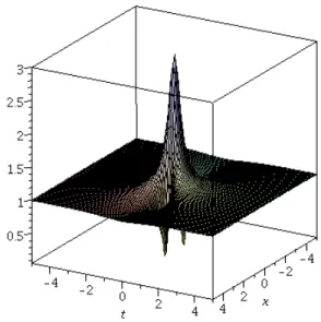
3/4 we get the Peregrine solution [9] : P1(x, t) =
1−4 1 + 4it 1 + 4x2+ 16t2
e2it≡
1−4 1 +iT 1 +X2+T2
eiT /2, X := 2x, T := 4t.
Its plot is presented in figure 1.
The case n = 2 is the first one where we get a family of solutions depending on 4 parameters including two nontrivial parametersϕ3 andϕ4. We already explained above that ϕ3 has a connection with the KP-I equation. For convenience we choose ϕ1 = 3ϕ3
andϕ2 = 2ϕ4+ (3 +√
5) sin(π/5)/4 and we switch from the pair of parameters {ϕ3, ϕ4} to the pair {α, β} defined by
α:= 48ϕ3
β:= 4(5 +√
5) sin(π/5)−96ϕ4. The solutions read
u2(x, t, α, β) =
1−12G(2x,4t) +iH(2x,4t) Q(2x,4t)
e2it (41)
where
G(X, T) := X4+ 6(T2+ 1)X2+ 4αX+ 5T4+ 18T2−4βT −3 H(X, T) :=T X4+ 2(T3−3T +β)X2+ 4αT X+T5+ 2T3
−2βT2−15T + 2β
Q(X, T) := (1 +X2 +T2)3−4αX3−12(2T2−βT −2)X2 + 4(3α(T2+ 1)X+ 6T4−βT3+ 24T2−9βT
+α2+β2+ 2). (42)
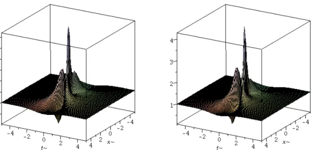
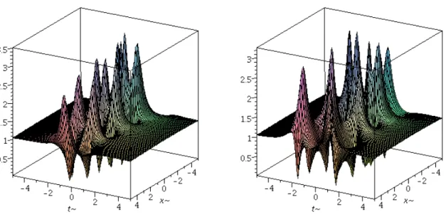
When α = β = 0 this solution coincide with the P2-breather with maximum of magnitude equal 5 obtained at the point x = t = 0. When α2 +β2 is small enough the solution is obviously very close to the P2-breather. Formula (42) shows that the solution u2(x, t, α, β) can be considered as a two-parametric quadratic deformation of the P2-breather. When the two parameters are large enough we obtain the ”generic”
form of rank 2 multi-rogue waves : three rogue waves of similar height. These two phenomenon are shown in figure 2. In between we can observe some transition states.
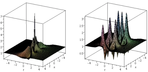
Some are represented in figure 3 or figure 4.
Formula (42) which was first discovered in [2, 3, 4] was very important, showing for the first time that, contrary to the genuine Peregrine breathers, its higher versions are not isolated.+ There exist a families of solutions with very similar properties (obtained by the sufficiently small variation of parametersα andβ in vicinity of their zero values) having almost the same extreme rogue wave behaviour as theP2-breather. Formula (42) also clearly answered the question posed by Eleonski and Kulagin about 28 years ago : how to embed the P2 breather discovered in [11] into a larger family of quasi rational solutions of the NLS equation.∗
+ In [2, 3, 4] the parametersα, βwere defined differently. They were proportional to those we use here in order to shorten the writing of the formulas.
∗ It is instructive to see the movies KP2a, KP2e providing at any fixed moment of time the plot of the square of the absolute value of the related solution of the NLS equation. See the subsection ”Links with KP-I equations and the related movies” below.
When α2 +β2 tends to ∞, u2(x, t, α, β) tends to e2it. Thus, a simple wave, i.e.
rank 0 solution, can be interpreted as a large parametric limit of the rank 2 multi-rogue wave solution. Below we will show that for higher ranks similar but more diversified phenomena take place.
Figure 1. The Peregrine solution
Figure 2. Second order solution (41) forα= 0 andβ= 0 on the left andα= 20 and β= 20 on the right
Figure 3. Second order solution (41) forα= 0 andβ = 1 on the left andα= 0 and β= 3 on the right
Figure 4. Second order solution (41) forα= 0 andβ = 6 on the left andα= 5 and β= 0 on the right
3.2. Rank 3 solutions
The ϕ-parametrization described above makes it difficult to isolate the values of parameters describing higher Peregrine breathers. Similarly to the previous section here we introduce 4 ”essential” parametersα1, β1, α2, β2. We chooseϕj according to the following linear system
ϕ1 = 3ϕ3−5ϕ5
ϕ2 = 2ϕ4−3ϕ6+4(1sin(π/7)−cos(π/7)) 768ϕ3 = 26α1−α2
1920ϕ4 = −40β1+β2+ 96(3 sin(π/7) + 8 sin(2π/7) + 2 sin(3π/7)) 3840ϕ5 = 10α1−α2
7680ϕ6 = −20β1+β2+ 32(4 sin(π/7) + 14 sin(2π/7) + sin(3π/7)).
Substituting these formulas in expression (15) for n = 3, we can after long calculation, using Maple, convert the related solution of NLS equation in the following explicit form :
u3(x, t, α1, β1, α2, β2) =
1−24G3(2x,4t) +iH3(2x,4t) Q3(2x,4t)
e2it (43) with
G3(X, T) = X10+ 15(T2+ 1)X8+P6
n=0gn(T)Xn H3(X, T) = T X10+ 5(T3−3T +β1)X8 +P6
n=0hn(T)Xn
Q3(X, T) = (1 +X2+T2)6−20α1X9−60(2T2−β1T −2)X8+ 4P7
n=0qn(T)Xn where
g6 = 50T4−60T2+ 80β1T + 210 g5 = 120α1T2−18α2+ 300α1
g4 = 70T6−150T4+ 200β1T3+ 450T2 + 30β2T −450 + 150α21−50β12 g3 = 400α1T4+ (3000α1−60α2)T2−800α1β1T −600α1−60α2
g2 = 45T8+ 420T6+ 6750T4−(6000β1−180β2)T3−(300α21 −900β12+ 13500)T2 +(3600β1+ 180β2)T −675−300α21 −300β12
g1 = 280α1T6+ (150α2−2100α1)T4+ 800α1β1T3−(3600α1−540α2)T2 +(120β2α1+ 1200α1β1−120α2β1)T −200α1β12−900α1−90α2 −200α31 g0 = 11T10+ 495T8−120β1T7+ 2190T6−(42β2+ 1200β1)T5
+(350α21+ 150β12−7650)T4+ (6600β1−420β2)T3
−(2100β12+ 2025−120β2β1−120α2α1+ 900α21)T2+ (200α21β1+ 200β13−90β2)T +675 + 150α21+ 6α22+ 150β12+ 6β22
h6 = 10T5−140T3+ 40β1T2−150T + 60β1−5β2
h5 = 40α1T3+ (60α1−18α2)T + 40α1β1
h4 = 10T7−210T5+ 50β1T4−450T3+ 15β2T2−(50β12+ 1350−150α21)T +150β1−15β2
h3 = 80α1T5+ (1000α1−20α2)T3−400α1β1T2−(1800α1−60α2)T +200α1β1+ 20β2α1 −20α2β1
h2 = 5T9−60T7+ 1710T5+ (45β2−2100β1)T4+ (300β12−6300−100α21)T3 +(1800β1−90β2)T2 + (4725 + 300α21+ 300β12)T −135β2−100β13
−100α21β1−900β1
h1 = 40α1T7+ (30α2−1140α1)T5+ 200α1β1T4−(2400α1−60α2)T3
+(60β2α1−60α2β1+ 600α1β1)T2−(900α1+ 450α2+ 200α13+ 200α1β12)T +60α2β1−60β2α1
h0 = T11+ 25T9−15β1T8−870T7+ (40β1−7β2)T6+ (70α21−9630 + 30β12)T5 +(5850β1−75β2)T4 + (40β2β1 + 40α2α1−2475−900α21−1300β12)T3 +(100α21β1+ 495β2+ 100β13)T2+ (6α22+ 4725−240α2α1−240β2β1
+750β12+ 6β22+ 750α21)T −20α21β2−675β1−45β2−100α21β1−100β13 +40α2α1β1 + 20β12β2
q7 = 3α2−30α1
q6 = −60T4+ 40β1T3+ 120T2−(15β2−60β1)T + 35β12+ 15α21+ 580 q5 = 30α1T4 −(27α2−90α1)T2 + 120α1β1T −27α2+ 540α1
q4 = 30β1T5−360T4+ (15β2+ 600β1)T3+ (3360 + 225α21−75β12)T2 +(135β2−1350β1)T + 225β12−30α2α1+ 525α12−30β2β1+ 840 q3 = 40α1T6 + (1950α1−15α2)T4−400α1β1T3+ (90α2+ 4500α1)T2
+(60β2α1−1800α1β1 −60α2β1)T −450α1+ 100α31+ 100α1β12−135α2 q2 = 60T8+ 3360T6−(1620β1−27β2)T5+ (225β12−75α21 + 19560)T4
−(16200β1 −270β2)T3 + (450α12−9120 + 4050β12)T2
+(675β2+ 2700β1−300β13−300α12β1)T + 3036 + 9α22−180α2α1
+225β12+ 225α21+ 9β22−180β2β1
q1 = 15α1T8 + (15α2−90α1)T6+ 120α1β1T5+ (405α2−5400α1)T4
+(3000α1β1−60α2β1 + 60β2α1)T3+ (1485α2−300α1β12−1350α1−300α31)T2 +(540β2α1−540α2β1)T + 300α31−120α1β1β2−60α2α21+ 135α2+ 60α2β12 +300α1β12+ 2025α1
q0 = 30T10−5β1T9+ 930T8−(240β1+ 3β2)T7+ (15β12+ 3820 + 35α21)T6 +(1710β1 −153β2)T5+ (30β2β1+ 30α2α1−975β12+ 35940−75α21)T4 +(100β13+ 100α21β1+ 135β2−23400β1)T3
+(9β22+ 23286 + 9α22−360β2β1−360α2α1 + 4725α12+ 8325β12)T2
+(120α2α1β1−60α21β2−1500α21β1 + 60β12β2−7425β1−675β2−1500β13)T +506 + 9β22+ 100β14+ 675α12+ 100α41+ 9α22+ 90β2β1+ 200α21β12
+675β12+ 90α2α1.
We can easily get the solutions of the first section by choosing the parameters α1 = 48(ϕ3−5ϕ5),
α2 = 480(ϕ3−13ϕ5),
β1 = 96(4ϕ6−ϕ4) + 8(sin(π/7) + 2 sin(2π/7) + sin(3π/7)), β2 = 1920(8ϕ6 −ϕ4) + 32(sin(π/7)−4 sin(2π/7) + 4 sin(3π/7)) and performing the translation x, t x−ϕ1, t−ϕ2.
It is easy to see that P3 can be obtained as u3(x, t,0,0,0,0) and in particular
|P3(0,0)| = 7. Let us indicate the particular values of ϕj corresponding to the P3 breather corresponding to particular solution of the system (3.2) withαj =βj = 0, j = 1,2 :
ϕ1 =ϕ3 =ϕ5 = 0,
ϕ4 = (3 sin(π/7) + 8 sin(2π/7) + 2 sin(3π/7))/20, ϕ6 = (4 sin(π/7) + 14 sin(2π/7) + sin(3π/7)/240, ϕ2 = 2ϕ4−3ϕ6+ sin(π/7)
4(1−cos(π/7)).
One of the advantage of this representation of the solution is that we can analyze its limit behavior when one or several parameters tend to infinity and x and t remain bounded.
• If α2 and β2 remain finite then u3(x, t, α1, β1, α2, β2) tends to e2it when α21 +β12 tends to ∞.
• Ifα1 and β1 remain finite thenu3(x, t, α1, β1, α2, β2) tends to P1(x, t) when α22+β22 tends to ∞.
• If α1, β1,α2 and β2 all tend to∞ in the following way β1 ∼bα1, α2 ∼cαr1, β2 ∼dαr1
then the limit ofu3(x, t, α1, β1, α2, β2) depends onraccording to the following table
r limit
<2 e2it
>2 u1(x, t) 2 u1(x−x1, t−t1) where x1 and t1 are defined by
x1 = 10(13(c−b22+d)c+20bd2) t1 = 10(13(c−b22+d)d−2)20bc
Thus we have shown that u3 contain the solutions of rank 0 and 1 as appropriate large parametric limits. Plots for several choices of parameters are shown in figure 5 and 6.
Figure 5. Third order solution (43) for α1 = β1 = α2 = β2 = 0 on the left and α1=β1=α2=β2= 50 on the right
Figure 6. Third order solution (43) forα1 =α2 = 0 and β1 =β2 = 50 on the left andα1=β1= 0 andα2=β2= 5000 on the right
3.3. Rank 4 solutions
Here we present without details the formulas providing the 6-parametric family of multi- rogue wave solutions similar to the one of the previous section :
u4(x, t, α1, β1, α2, β2, α3, β3) =
1−40G4(2x,4t) +iH4(2x,4t) Q4(2x,4t)
e2it (44) with
G4(X, T) = X18+ 27(T2+ 1)X16−24α1X15+P14
n=0gn(T)Xn H4(X, T) = T X18+ 9(T3−3T +β1)X16−24α1T X15+P14
n=0hn(T)Xn Q4(X, T) = (1 +X2+T2)10−60α1X17−180(2T2−β1T −2)X16+ 4P15
n=0qn(T)Xn. The interested reader can find the explicit formulas for the coefficients in appendix.
These solutions are polynomials of order 6 with respect to α1 and β1, of order 4 with respect toα2, β2 and quadratic with respect to α3, β3. TheP4-breather is obtained from it by setting αj = βj = 0,∀j. It is easy to see that |P4(0,0)| = 9. As above we can investigate the limit of this solution when one or several parameter tends to infinity and x and t remain bounded.
• Ifα2, β2,α3 and β3 remain finite thenu4(x, t, α1, β1, α2, β2, α3, β3) tends to P1(x, t) when α21+β12 tends to∞.
• If α1, β1, α3 and β3 remain finite then u4(x, t, α1, β1, α2, β2, α3, β3) tends to e2it when α22+β22 tends to∞.
• If α1, β1, α2 and β2 remain finite then u4(x, t, α1, β1, α2, β2, α3, β3) tends to u2(x, t, α1, β1) when α23+β32 tends to∞.
• Ifα3 and β3 remain finite and α1, β1,α2 and β2 all tend to ∞ in the following way β1 ∼bα1, α2 ∼cαr1, β2 ∼dαr1
then the limit of u4(x, t, α1, β1, α2, β2, α3, β3) depends onr according to the follow- ing table
r limit
<3/2 u1(x, t)
>3/2 e2it
3/2 u1(x−x2, t−t2) where x2 and t2 are defined by
x2 = 3((1−3b2)(d50(b2−2c2+1))+2(b3 2−3)bcd) t2 = 3((3−b2)b(d50(b2−c22+1))+2(13 −3b2)cd).
• Ifα2 and β2 remain finite and α1, β1,α3 and β3 all tend to ∞ in the following way β1 ∼bα1, α3 ∼eαs1, β3 ∼f αs1
then the limit of u4(x, t, α1, β1, α2, β2, α3, β3) depends ons according to the follow- ing table
s limit
<2 u1(x, t)
>2 e2it
2 u1(x−x3, t−t3) where x3 and t3 are defined by
x3 = (2bf+(135(b2+1)−b22)e) t3 = (2be35(b−(12+1)−b22)f).
• If α1 and β1 remain finite andα2,β2, α3 and β3 all tend to ∞ in such a way that β2 ∼dα2, α3 ∼eαp2, β2 ∼f αp2,
then, the limit of u4(x, t, α1, β1, α2, β2, α3, β3) depends onpaccording to the follow- ing table
p limit
<2 e2it
>2 u2(x, t, α1, β1) 2 u2(x, t, α1−α0, β1 −β0) where α0 and β0 are defined by
α0 = 21(2df+(110(e2+f−2d)2)e)
β0 = 21(2de10(e−2(1+f−d2)2)f).
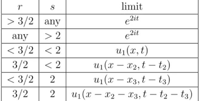
• If α1, β1,α2,β2, α3 and β3 all tend to ∞ in the following way β1 ∼bα1, α2 ∼cαr1, β2 ∼dαr1, α3 ∼eαs1, β3 ∼f αs1.
then the limit of u4(x, t, α1, β1, α2, β2, α3, β3) depends on r and s according to the following table
r s limit
>3/2 any e2it
any >2 e2it
<3/2 <2 u1(x, t) 3/2 <2 u1(x−x2, t−t2)
<3/2 2 u1(x−x3, t−t3) 3/2 2 u1(x−x2−x3, t−t2−t3) where x2, t2, x3 and t3 are defined as above.
It seems that un contain all solutions of order 0 to n−2 as appropriately chosen large parametric limits. Of course for higher ranks further work has to be produced to get the similar results. In figure 7 to 9 we present some plots of fourth order solutions.
Figure 7. Fourth order solution (44) forα1=β1=α2=β2=α3=β3= 0
Figure 8. Fourth order solution (44) forα1=β1 =α2 =β2=α3=β3 = 20 on the left andα1=β1= 0 and α2=β2=α3=β3= 1500 on the right
Figure 9. Fourth order solution (44) for α1 =β1 =α2=β2= 0 andα3=β3= 105 on the left andα1=β1= 20,α2=β2= 0 andα3=β3= 105on the right
3.4. Links with the KP-I equation and the related movies
Assume now that B = 1 andϕj, j 6= 3 are selected in such a way that when t= 0 un(x, y, ϕ1, ϕ2,0, ϕ4, . . . , ϕ2n) =Pn(x, y).
Then the related solution of the KP-I equation attains its absolute maximum at the point x=t =y = 0 and
v(0,0,0) = 2[(2n+ 1)2−1] = 8n(n+ 1).
For instance for n= 2 this corresponds to ϕ1 = 0, ϕ2 = (7 + 5√
5)sinπ/5
6 , ϕ4 = (5 +√
5)sinπ/5
24 . (45)
Therefore similarly to the P2-breather the solution of the KP-I equation vp2(x, y, t) generated by the selection of the phases above is rigid. It attains at the point x = y = t = 0 the absolute maximum v(0,0,0)=48. This maximum is 3 times greater then the height of the KP-I image of the P1 breather.
Quite similarly, for the case n= 3, from the formulas (44) we see that selecting the phases as
ϕ1 =ϕ5 = 0, ϕ3 =−t,
ϕ4 = 3 sin(π/7) + 8 sin(2π/7) + 2 sin(3π/7)/20, ϕ6 = (4 sin(π/7) + 14 sin(2π/7) + sin(3π/7)/240, ϕ2 = 2ϕ4−3ϕ6+ sin(π/7)
4(1−cos(π/7)) (46)
we obtain via the same formula (22) the smooth rational solution of the KP-I equation which we denotevp3(x, y, t) such thatvp3(0,0,0) = 96. The related maximum is 6 times higher then the KP-I image of theP1-breather.
These solutions of the KP-I equation can also be obtained from the α, β parametrization of the solutions of the NLS equation. Investigating the relation be- tween the parameters ϕj and the parameters αj, βj shows that performing the changes of variables t y, x x+ 3t, α1 −48t and α2 −480t +γ where γ is a free real parameter is equivalent to the transformation presented above. It gives us a fam- ily of solutions depending on one parameter β1 in the case n = 2 and three parameters β1, β2, γ in the casen= 3 that differ from the families constructed above by translations inx, y, t. The time evolution of some of these solutions can be observed on the 5 movies available at http://www.kurims.kyoto-u.ac.jp/ kirillov/MATVEEV.
The first movie KP2a shows the triangular configuration of 3 peaks corresponding to the choice of parameters β1 = 20 which at the moment of their appearance have
˜
the average height 16. At the large negative times it is close to an isosceles triangle of growing size when t → −∞. Close to t = 0 the triangle loses its form and rotates while propagating so that the peaks do not produce the confluence but rather the peak, initially coinciding with the left vertex of the back side of the triangle, after some rotation acquires the maximal height 25 at the moment when the distances between the peaks are minimal. After this the peaks diverge forming asymptotically at large times an isosceles triangle of growing size.
For the second movie (KP2e) with β1 = 0 the scenario is different. The initial triangle (again almost isosceles for large negative times) does not rotate and contracts progressively so that first happens the confluence of two peaks situated behind a first one going ahead. Next, the so formed higher peak approaches the slower and smaller one, so that at the moment of their confluence they form one peak of the height 48, surrounded by four small peaks.] After the full confluence the mirror image of the previous configuration appears forming asymptotically the isosceles triangle of growing size .
The next three movies represent the evolution of a triangular array containing 6 peaks forming for large negative times the almost isosceles triangle. The first of them (KP3a) with β1 = 20, β2 = 20, γ = 0 behaves as follows. First for large negative times we have the almost isosceles triangular array containing 6 peaks. When t → 0, t < 0 the triangle rotates and contracts arriving to the maximal height 35 at some moment of time with no confluence between peaks after which it starts to diverge again forming at large positive times the configuration close to an isosceles triangle. For the second movie KP3b with β1 = 0, β2 = 20, γ = 0 the maximum of amplitude in the ”collision area” is a bit higher but still there is no total confluence of 6 peaks. Finally, in a third movie (KP3e) with β1 = 0, β2 = 0, γ = 0 we see the formation of the extremal rogue wave of the height 96 reaching at the moment t= 0 absolute maximum of the solution located at the point (x, y) = (0,0).
It is worthwhile to mention that, taking into account the NLS-KP correspondence (22) the presented movies also show the infinite numbers of space time plots for the square of magnitude of the NLS multi rogue wave solutions of the ranks 2 and 3 in particular illustrating a variety of important non symmetric configurations including 2 peaks configurations.
4. Concluding remarks
1. Our works [1, 2, 3, 4] were the first to explain the concept of the multiple-rogue waves solutions and their links with higher order Peregrine breathers thus, in particular, answering a question posed by Eleonski and Kulagin almost 30 years ago : how to incorporate the second order Peregrine breather discovered in [11] to the larger family of rational solutions. The work [5] was written in 1986 exactly for this purpose but it
] this already gives an idea of what is an extremal rogue wave solution of the KP-I equation.
was not properly understood until the appearance of our works written in 2010-2011.††
The explanation of the related formula (15) for the multi-rogue waves solutions takes less than one page and contains all necessary definitions. This formula is of about the same length with respect to other recently appeared works and it was the first which allowed to understand that generic multi-rogue wave solutions (unknown before) can be considered as a simple rational (with respect to free parameters) deformations of the higher Peregrine breathers or Pn breathers as we call them here. In addition this formulation has the advantage of providing the natural construction of the multi-rogue waves smooth rational solutions of the KP-I equation. By a way these solutions are quite different from the so called multi-lumps smooth rational solutions of the KP-I equation found in 1977 in [12]. Already in our first work [1] we mentioned that a number of other approaches namely Darboux transformation formulas for the NLS equation (known since 1882, see for instance [8, 13, 14]) and also a passage to appropriate infinite periods limit in multi-periodic solutions (first obtained in [10, 15] via degeneration of finite gap multi- periodic solutions) should provide another description of the same multi-rogue wave solutions. This prediction was fully realized for DT approach by Guo, Ling and Liu [16] and for the other mentioned approach it was done (to some extent) by P. Gaillard [17, 18, 19, 20]. In these works another formulas for the multi-rogue waves solutions were obtained producing for all tested ranks the higher Peregrine breathers just setting all the parameters to be zeros. In particular, in 2011-2012 Pierre Gaillard computed all the Pn breathers of the rank n≤10. Before that, only the genuine Peregrine breather, the P2-breather found in 1985 and theP3-breather discovered in 2009 [21, 22] were explicitly described.
2. In addition, Hirota direct method was successfully applied to obtain also the description of the multiple rogue waves solutions by Ohta and Yang [23]. The multi- rogue wave solutions in [23] were expressed as a ratio of two tau-functions polynomial with respect to complex parameters aj, aj. In their work the authors considered the complex conjugate of the NLS equation and Gross-Pitaevskii equation used here. For their form of the GP equation they obtained a beautiful explicit formula (3.20) in which dominator and denominator of the solution are polynomials of the complex parameters am, am, a0 = 1, a2j = 0,∀j ≥1.For particular values of their parameters Ohta and Yang first detected, for the rank 3 solutions, not only the circular arrays found slightly before [18, 19, 24] but also the configurations of the six peaks forming a triangular array close to an equilateral triangle with a slightly curved base (concave or convex) depending on the choice of parameters (see the figure 2 of [23]). This was an indication that the solutions discussed in [17, 18, 24, 25] were not generic contrary to our works [1, 2, 3, 4] and the works [16] and [23]. Our films (see the reference on the related URL above) show that the evolution of these triangular configurations is responsible for formation of extreme rogue waves events described by KP-I equations and provide for ranks 2 and 3 an infinite
††That’s true that every of the formulas describing the multi-rogue wave solutions including our works [1, 2, 3, 4] and those which appeared later [16, 23] , [19] have there own advantages and disadvantages and quite a different analytic and combinatorial structures.
number of such triangular configurations from the point of view of NLS equation. Some triangular static configurations were also found slightly later with respect to [23] by Guo, Ling and Liu [16] using their approach based on Darboux transformation. In [16]
similar triangular structure was also first found for the Hirota equation.
3. One further comment concerns two more points in the work by Ohta and Yang.
In [23] the values of parameters leading to the higher Peregrines breather were pointed out only for ranks n = 1,2,3. The connection between the real parameters αj and βj
used above and the complex valued parametersaj used in [23] forj = 2,3,4 is given by the formulas
12a3 =α1−1−iβ1, 240a5 =α2−1−iβ2, 10080a7 =α3 −1−iβ3.
In general the passage from the variables αj, βj to the variables aj of [23] is given by the formula
a2j+1 = αj−1−iβj
2(2j+ 1)! . (47)
One of us (Ph. Dubard) conjectured that as all Pn-breathers with the maximum of magnitude located at the point x = −1/2, t = 0 in the approach of [23] correspond to the choice ofaj given by (47) with αj =βj = 0 i.e.
a2j+1 =− 1
2(2j+ 1)!, j ≤n, aj = 0 ∀j ≥2n+ 2. (48) This conjecture was confirmed by Ph.Dubard for the ranks n≤7 although the general proof is still missing .
Ohta and Yang also detailed their formula (3.20) expressing the matrix elements of the related determinants by means of Schur polynomials with the arguments containing some rational numbers rk, sk defined by means of simple generating functions (see the formulas (4-9) of [23]), satisfying the conditionr2k+1 =s2k+1 = 0. The short calculation proves thatr2k, s2k are simply expressed by means of Bernoulli numbersB2n. The laters are defined by the formula
t et−1 =
∞
X
n=0
Bntn
n! . (49)
It follows from the definition above that B2n+1 = 0,∀n≥1.
Now it is easy to prove the formulas:
r2n= (22n−1)
2n(2n)!B2n, s2n=−22n−2
2n(2n)!B2n, r2n+s2n= B2n
n(2n!). (50) Since all Bernoulli numbers are rational this proves that it is also true forskandrk. Also taking into account that Bernoulli numbers are very well studied this gives a simplest way to compute r2j, s2j.
4. Another important comment concerns the works of Pierre Gaillard [17, 18, 19, 20]
and several others deposed on Arxiv hal. The key idea of these works suggested by one of us (VM) in 2010 was to obtain the multi-rogue waves solutions considering an
appropriate passage to the limit in the formulas describing the multi-phase trigonometric modulations of the plane wave solutions [10, 15]. In fact in all of these works by P. Gaillard despite the apparent presence of 2n or even more free parameters (for the rank n) the related solutions were always 2 parametrical as we will briefly explain below.
The reason to think so was the absence in his plots of the triangular arrays similar to those appearing already for n = 3 in [16] and [23]. Therefore we asked the author to print out the related analytical expressions for ranks 3,4 and 5 including explicitly all his parameters aj, bj. At that time we already have got a formulas equivalent to α, β parametrisation of this article for n=3 and 4. The comparison of Gaillard solutions with ours shown that they are:
1. Simply equivalent to solutions of this work with α1, β1 = 0 for n = 3 and to the solutions of this work for n = 4 with α1 =α2 =β1 =β2 = 0.
2. As we explained to Gaillard his solutions in fact are equivalent to those obtained from his own formulas by setting for instance aj = bj = 0 ∀j > 1 . One of us (VM) showed that this can be proved in intrinsic terms: first of all for any rank n it can be checked that all the terms in numerators and denominators of his formulas are just the quadratic polynomials of the same linear combinations ofaj orbj, and such a structure can not correspond to generic rational solution for the rank greater then 2. For instance, for one of the works of PG for rank 4 these linear combinations found by VM are:
a= (a1+ 26a2+ 36a3−212a4), b = (b1+ 26b2+ 36b3−212b4).
All coefficients depending on the parameters in this case are proportional to a2 +b2 or to a and b. This was also checked for higher ranks but of course the coefficients in the aforementioned linear combinations are depending on the rank but qualitatively the fact rest the same. All the formally multi-parametric solutions of the works by Gaillard of the period 2011-2012 were dealing with two parametric quadratic deformations of the higher Peregrine breathers. The work [19] was written already on the base of this understanding which allowed to compactify drastically his previous calculations.
Unfortunately he never explained clearly all these points. Therefore the history of coming to modern understanding explained above, which was asking a big amount of work and intelligent study of monstrous formulas obtained as a Maple output having volumes of hundreds of pages already for n=5, was never explained to the reader before.
Quite recently in [20] he succeeded to produce, by taking a new kind of long periods limit of [10] a full family of the rank 3 solutions. Initially he supposed that he found a new solution. In fact it is the same solution which he learned from us already in March 2012, corresponding to the formula (43). Exact correspondence between these two solutions computed by Ph. Dubard reads as follows :
a1 =−α1
2 , b1 =−β1
2, a2 = 60α1−6α2, b2 = 83
2 β1−6β2.
Of course this latest result of PG means that in general the method of passage to the limit in [10, 15] produces also the generic solutions under appropriate choice of the limiting procedure but further work in this direction for higher ranks should be done.