A numerical verification method for solutions of initial value problems for ODEs
using a linearized inverse operator
By
Takehiko KINOSHITA, Takuma KIMURA, and Mitsuhiro T. NAKAO
June 2012
R ESEARCH I NSTITUTE FOR M ATHEMATICAL S CIENCES
KYOTO UNIVERSITY, Kyoto, Japan
A numerical verification method for solutions of initial value problems for ODEs using a linearized inverse operator
Takehiko Kinoshita · Takuma Kimura · Mitsuhiro T. Nakao
June 7, 2012
Abstract We propose a new verification method to enclose solutions for initial value prob- lems of systems of first-order nonlinear ordinary differential equations (ODEs) using a lin- earized inverse operator. The proposed approach can verify the existence and local unique- ness of the exact solution independent of the choice of the approximation scheme, while the existing methods usually depend on the numerical scheme for the approximate solution.
In contrast, most of the well-known verification methods to enclose solutions for nonlinear ODEs work only on the specified approximate solution. Namely, in the existing verification methods the numerical scheme for computing an approximate solution is essentially limited to the Taylor method . Therefore, one of our purposes is to develop a verification method that can obtain guaranteed error bounds independent of the approximation scheme. We will present numerical examples of the proposed verification method that obtain rigorous er- ror bounds of the approximate solutions obtained by the Euler method or the second-order Runge-Kutta method.
Keywords Nonlinear ODEs·Initial Value Problems·Finite Difference Method·Finite Element Method·Numerical Verification Method
Mathematics Subject Classification (2000) 34A34·65L05·65L12·65L60·65G20
1 Introduction
In this paper, we consider a numerical verification method for the existence and the local uniqueness of solutions for the following system of first-order nonlinear ordinary differential
Takehiko Kinoshita
Research Institute for Mathematical Sciences, Kyoto University, Kyoto 606-8502, Japan E-mail: [email protected]
Takuma Kimura
JST CREST / Faculty of Science and Engineering, Waseda University, Tokyo 169-8555, Japan E-mail: [email protected]
Mitsuhiro T. Nakao
Sasebo National College of Technology, Nagasaki 857-1193, Japan E-mail: [email protected]
equations (ODEs):
{ Au0=f(t,u), in J, (1a)
u(0) =u0, (1b)
whereu:= (u1, . . . ,un)Tis ann-dimensional vector function. Here,J:= (0,T)⊂R,(T<∞) is a bounded interval,nis a positive integer,Ais a symmetric positive-definite matrix in Rn×n,u0is an arbitrary initial vector in a given initial-value setU0⊂Rn, andfis a nonlinear operator fromJ×Lp(J)ntoL2(J)n,(2≤p≤∞). In addition, we assume that f is Fr´echet differentiable at an arbitraryv∈H1(J)n and the derivative f0(v)belongs toL∞(J)n×n. We denote that the solutionu(t)of (1a) and (1b) asu(t;u0). An orbit of (1a) starting atu0 is given by the setγ(u0):={
u(t;u0)∈Rn;t∈J}
, whereJ:= [0,T]means the closure ofJ.
Moreover, we define the family of the orbit of (1a) and (1b) as the union of the orbits for all initial values, i.e.,γ(U0):=∪u0∈U0γ(u0).
Many methods have been developed for the same purpose. The Lohner method [6] and the Taylor model developed by Berz and Makino [1] are especially well known. Moreover, various software packages exist, including AWA by Lohner [7] and COSY INFINITY by Makino [8]. RiOT and ACETAF by Eble [2] are also available. A technique combining the Taylor model [1] and Nakao’s method was proposed by Yamamoto and Komori [11]. All of these existing works are verification methods for the orbits of nonlinear ODEs that use the Taylor series. Therefore, the nonlinear operator fmust be smooth enough fortandu.
In contrast, our method is based on functional analysis, and it does not need the higher- order derivatives of f. Moreover, we only need an approximate solution, which can be cal- culated by any algorithm. Therefore, our method can be applied to a much wider range of mathematical problems than those for which previous methods are appropriate. Also, some of the numerical results in Section 8 show that the present approach gives better accuracy than the existing method.
2 Notation and function spaces
In this section, we introduce the function spaces and the projections onto finite-dimensional subspaces that will be used in this paper. LetL2(J)be the set of square integrable func- tions onJ, which is a real Hilbert space with inner product(u,v)L2(J):=∫Ju(t)v(t)dt. For arbitrary 1≤q<∞, letLq(J)be a Banach space with norm kukLq(J):= (∫J|u(t)|qdt)1q. Similarly, letL∞(J)be a Banach space with normkukL∞(J):=ess supt∈J|u(t)|. For each u∈Lq(J)n, we defineNq(u)∈RnasNq(u):=
(ku1kLq(J), . . . ,kunkLq(J)
)T
. LetH1(J)be a Sobolev space defined byH1(J):={
u∈L2(J);u0∈L2(J)}
, which is a Hilbert space with inner product (u,v)H1(J):= (u,v)L2(J)+ (u0,v0)L2(J). LetV1(J)be a subspace ofH1(J)defined byV1(J):={
u∈H1(J);u(0) =0}
. Then,V1(J)is a Hilbert space with inner product(u,v)V1(J):= (u0,v0)L2(J).
For a Banach spaceXand a positive integern, we define then-dimensional Banach space XnbyXn:=X×···×Xwith normkukXn:=
√
∑ni=1kuik2X. Similarly, letXn×nbe ann-by-n matrix Banach space. We denote theL∞(J)n×nnorm bykBkL∞(J)n×n:=ess supt∈Jmax
√σ(
B(t)TB(t)) , whereσ(
B(t)TB(t))
⊂Rare the set of eigenvalues forBTB.
For arbitrary 1≤q<∞, we define the`q norm forx∈Rn bykxk`q := (∑ni=1|xi|q)1q. Moreover, we define the`∞norm forx∈Rnbykxk`∞:=max{|x1|, . . . ,|xn|}.
LetHk1(J)nbe a finite-dimensional subspace ofH1(J)nwherek>0 is the discretization parameter.
We denote the set of floating-point numbers by F. For the nonsingular floating-point number matrixM∈Fn×n, the interval vector[ξ]⊂Rn, which includes 0, and the translation vectorζ∈Fn, we define the initial-value setU0⊂RnasU0=ζ+M[ξ]. Namely, we assume that the initial-value set is represented by an affine map in our verification method.
3 Numerical solutions
From the definition ofU0,ζ is an element ofU0. Therefore, we defineuk∈Hk1(J)nas the approximate solution of (1a) and (1b) that approximately satisfies the following nonlinear ODEs:
{ Au0k=f(t,uk), in J, (2a)
uk(0) =ζ. (2b)
Namely, it is sufficient to satisfy the equality of (2a) in the approximate sense, but we as- sume that the equality (2b) is rigorously satisfied. Moreover, we can use any algorithm to solve (2a) numerically. Namely, the calculation to obtainukcould be done by floating-point number operations, and we do not need any rigorous computations that would yield the exact solution of (2a). However,ukhas to be an element ofHk1(J)n.
For example, when (2a) and (2b) are solved by the finite difference method, no round- ing errors are generated in the calculation ofuk(0) =ζ becauseζ∈Fn. Therefore, we can consider that the equality (2b) strictly holds. Since the finite difference method provides in- formation only at discrete points of the approximate solution, one has to use some suitable interpolation method to connect between these discrete points. It might be appropriate to chooseHk1(J)nas a Lagrange-type finite-element space that has the same order of conver- gence as the finite difference method.
4 Numerical fundamental matrix of solutions
From the definition of the initial-value setU0, for an arbitrary initial valueu0∈U0 there existsξ∈[ξ]such thatu0=ζ+Mξ. Here,ζis the center ofU0, andMξis the error for the initial valueu0. In Section 3, we defined the time evolution ofζin our verification method.
In this section, we will define the time evolution forMξ.
Sinceξis the “error”, it cannot be strictly expressed in a computer. Therefore, we con- sider the time evolution ofM. Note thatξ is an element ofRnand is not an interval ofRn. The interval vectors are notated by square brackets,[·], throughout this paper.
LetEk∈Hk1(J)n×nbe the approximate fundamental matrix of solutions that satisfies the following linear ODEs:
{ AEk0−f0(uk)Ek=0 in J, (3a)
Ek(0) =M. (3b)
Notice that, similar to the case ofuk, it is sufficient to approximately satisfy the equality (3a). However, the equality (3b) must be rigorously satisfied. In order to computeEk, it is usually appropriate to apply the same numerical method as foruk.
We now define the time evolution ofMξ byEk(t)ξ. Therefore, we can obtain the en- closure of this for anyξ ∈[ξ]byEk(t)[ξ], whereEk(t)[ξ]denotes the multiplication of a matrix and an interval vector.
5 Norm estimates for numerical solutions
In this section, we consider the estimates ofEk. For any 1≤q≤∞andi∈ {1, . . . ,n}, we defineNq(Ek,i)∈Rnby the vector whose elements consist of theLq(J)norm of thei-th row ofEk, i.e.,
Nq(Ek,i):=(Ek,i,1
Lq(J), . . . ,Ek,i,n
Lq(J)
)T
.
Lemma 5.1 For any1≤q≤∞and i∈ {1, . . . ,n}, the following estimate holds:
sup
ξ∈[ξ]
(Ekξ)
i
Lq(J)≤Nq(Ek,i)
`q sup
ξ∈[ξ]
kξk
`
q−1q . (4)
Proof. —— For arbitraryξ∈[ξ], we setus(t;ξ):=Ek(t)ξ. Then, thei-th component ofus
is written byus,i(t;ξ) =∑nj=1Ek,i,j(t)ξj.
First, we consider the case of 1<q<∞. From the H¨older inequality, we have kus,i(·;ξ)kqLq(J)=
∫ J
∑
n j=1Ek,i,j(t)ξj
q
dt
≤∫
J
( n
∑
j=1Ek,i,j(t)q)(
∑
n j=1ξjq−1q )q−1
dt
= ( n
∑
j=1Ek,i,jqLq(J))(
∑
n j=1ξjq−1q )q−1
kus,i(·;ξ)kLq(J)≤Nq(Ek,i)
`qkξk
` q−1q .
Next, in the case ofq=1, we have kus,i(·;ξ)kL1(J)=
∫ J
∑
n j=1Ek,i,j(t)ξj
dt
≤ ( n
∑
j=1Ek,i,j
L1(J)
)
max{|ξ1|, . . . ,|ξn|}
=N1(Ek,i)
`1kξk`∞. Finally, in the case ofq=∞, we have
kus,i(·;ξ)kL∞(J)=ess sup
t∈J
∑
n j=1Ek,i,j(t)ξj
≤max{Ek,i,1L∞(J), . . . ,Ek,i,nL∞(J)} n
∑
j=1ξj
=N∞(Ek,i)
`∞kξk`1. Therefore, this proof is completed.
The upper bounds of supξ∈[ξ]kξk
`
q−1q in the right-hand side of (4) can be computed by interval arithmetic. Note thatEkis approximately computed, but the upper bounds of the norm ofEkmust be rigorously computed.
Similarly, the residual norm ofEkξis obtained as follows.
Lemma 5.2 For any1≤q≤∞and i∈ {1, . . . ,n}, the following estimate holds:
sup
ξ∈[ξ]
((AEk0−f0(uk)Ek
)ξ)
i
Lq(J)≤Nq((
AEk0−f0(uk)Ek
)
i)
`q sup
ξ∈[ξ]kξk
`
q−1q . (5) The proof is almost the same as that for Lemma 5.1, so we have omitted it.
Since the left-hand side of (5) is the residual norm ofEkξ, we expect that it has a conver- gence order with respect to the discretization parameterk. However, if we directly compute it by interval arithmetic, the convergence order may not be observed. This phenomenon is considered to be due to the cancellation of significant digits. On the other hand, the estimate of the right-hand side of (5) is separated into the interval[ξ]and the residual norm ofEk, which is independent of[ξ]. It plays an essential role in attaining the desired convergence order with respect to the discretization parameterk.
6 Verification conditions of solutions for the residual equation
We defined the approximate solution and the approximate fundamental matrix of solutions in Section 3 and Section 4, respectively. However, the discretization error, the truncation error, and the rounding error of (2a) and (3a) were not considered. We will discuss these errors in the present section using the residual equation.
Letξbe an arbitrary element of[ξ]. Then, the residual equation forξ is defined by { Aw0−f0(uk)w=f(
t,uk+Ekξ+w)
−f0(uk)w−Auk0−AEk0ξ,in J, (6a)
w(0) =0. (6b)
From now on, we will denote the right-hand side of (6a) bygξ(w):= f(
t,uk+Ekξ+w)
− f0(uk)w−Auk0−AEk0ξ. Moreover, we will denote the solutionw(t)of (6a) and (6b) by w(t;ξ). Then, the existence and the local uniqueness of the solutionu(·;u0)for (1a) and (1b) are equivalent to the existence and the local uniqueness of the solutionw(·;ξ)for (6a) and (6b). If we putu(t;u0):=uk(t) +Ek(t)ξ+w(t;ξ), thenu(·;u0)satisfies (1a). Also, from (2b) and (3b), we obtain the following equality:
u(0;u0) =uk(0) +Ek(0)ξ+w(0;ξ) =ζ+Mξ∈U0.
Therefore, in what follows, we consider the existence and the local uniqueness of the solu- tionw(·;ξ)for (6a) and (6b).
LetLt:V1(J)n→L2(J)nbe the linear ordinary differential operator of the left-hand side of (6a), i.e.,Lt:=Adtd −f0(uk). Then, the residual equations (6a) and (6b) are equivalent to the following fixed-point problem:
w(·;ξ) =Lt−1gξ( w(·;ξ))
. (7)
We denote the nonlinear integral operator of the right-hand side of (7) byFξ :=Lt−1gξ. Then, from the Sobolev embedding theorem, Fξ is a compact operator from Lp(J)n to Lp(J)n. Therefore, we can use the Schauder fixed-point theorem to show the existence of a fixed point of (7).
For a suitable positive constantα∈R, which is independent ofξ but which is deter- mined to be dependent on the interval vector[ξ], we define the candidate setWα⊂Lp(J)n as follows:
Wα:=
{
w∈Lp(J)n;kwkLp(J)n≤α} .
IfWαsatisfiesFξ(Wα)⊂Wα, then at least one fixed point of (7) exists inWαby the Schauder fixed-point theorem. Therefore, the sufficient condition ofFξ(Wα)⊂Wαbecomes a verifi- cation condition for the existence of a solution.
We assume that we can obtain the positive constantCL2,Lp that satisfies the following estimates:
Lt−1
L(
L2(J)n,Lp(J)n)≤CL2,Lp. (8) For example, a computational method to getCL2,Lp is given in [5]. Then, we have the fol- lowing estimates:
Fξ(Wα)
Lp(J)n= sup
w∈Wα
Lt−1gξ(w)
Lp(J)n
≤Lt−1
L(
L2(J)n,Lp(J)n) sup
w∈Wα
gξ(w)
L2(J)n
≤CL2,Lp sup
w∈Wα
gξ(w)
L2(J)n.
Therefore,Fξ-invariance ofWαis written as the the following inequality:
CL2,Lp sup
w∈Wα
gξ(w)
L2(J)n≤α. (9)
Since the parameterξis an arbitrary element of[ξ], we have the sufficient condition of (9) by
CL2,Lp sup
ξ∈[ξ]
sup
w∈Wα
gξ(w)
L2(J)n≤α. (10)
The rigorous upper bounds of supremum forξ in (10) can be computed by interval arith- metic. Thus, we can obtain the verification condition of the existence for the family of solu- tions with all initial data in[ξ].
Similarly, we can obtain the verification condition of the local uniqueness for solutions of the residual equation. Letξ be an arbitrary element of[ξ]⊂Rn. For a suitable positive constantγ∈R, ifWγhasFξ-contractility, then the fixed point ofFξ is unique inWγ. Namely, we show that there exists a constant 0≤CFξ <1 satisfying
Fξ(w)−Fξ(w)˜
Lp(J)n≤CFξkw−wk˜ Lp(J)n, ∀w,w˜∈Wγ. (11) Since the parameterξ is an arbitrary element of[ξ], we have the verification condition, 0≤supξ∈[ξ]CFξ <1, for the local uniqueness of the solution of the residual equation for arbitrary initial data in[ξ].
Remark 6.1 From the fact that the matrix A is symmetric and positive definite, it is seen that the initial value problems(1a)and u0=A−1f(t,u)are equivalent. Therefore, without loss of generality, we may assume that A is an identity matrix. However, from our experience on the estimates of the linearized inverse operator [5], the estimates of the inverse of Adtd −f0(uk) are usually easier than the estimates of the inverse of dtd −A−1f0(uk). This is because in the estimates for the inverse of Adtd −f0(uk), it is sufficient to get a lower bound of the minimum eigenvalue of A, while we need the square of the minimum eigenvalue of A for the estimate of the inverse of dtd −A−1f0(uk).
7 A posteriori estimates
After verifying the existence of a fixed point of (7), we calculate the a posteriori (error) estimates for the fixed point (i.e., the solution of (6a) and (6b)).
Theorem 7.1 Letα be a positive constant satisfying(10). For an arbitrary initial value u0∈U0, we denote the solution of(1a)and(1b)by u(·;u0)∈H1(J)n. Then, for any1≤q≤
∞and i∈ {1, . . . ,n}, we have the following error estimate:
sup
u0∈U0
ui(·;u0)−uk,i
Lq(J)n≤CL2,LqCL−21,Lpα+Nq(Ek,i)
`q sup
ξ∈[ξ]
kξk
`
q−1q . (12) Proof. —— From the definition ofU0, there existsξ∈[ξ]such thatu0=ζ+Mξ. Moreover, w(·;ξ)exists inWα, which is the fixed point of (7) forξ by assumption (10). Therefore, calculatingLqnorm for (7), we have
kwi(·;ξ)kLq(J)≤ kw(·;ξ)kLq(J)n
=Lt−1gξ(
w(·;ξ))
Lq(J)n
≤CL2,Lqgξ(
w(·;ξ))
L2(J)n
≤CL2,Lq sup
ξ∈[ξ]
sup
w∈Wα
gξ(w)
L2(J)n
≤CL2,LqC−L21,Lpα. From the fact thatu(t;u0) =uk(t) +Ek(t)ξ+w(t;ξ), we have
ui(·;u0)−uk,i
Lq(J)≤ k(Ekξ)ikLq(J)+kwi(·;ξ)kLq(J)
≤CL2,LqCL−21,Lpα+Nq(Ek,i)
`q sup
ξ∈[ξ]
kξk` q−1q ,
where we used Lemma 5.1.
From the result in Theorem 7.1 withq=∞, we obtain the enclosure of the family of the orbit of (1a) and (1b) as follows:
γ(U0)⊂ {
uk(t) +c∈Rn;t∈J, |ci| ≤CL2,L∞C−L21,Lpα+N∞(Ek,i)
`∞ sup
ξ∈[ξ]
kξk`1
}
. (13)
In order to verify solutions for the initial value problem step-by-step in time, it is very important to obtain the enclosure of the range of the family of solutions atT, i.e., the set{u(T;u0)∈Rn; u0∈U0}. This enclosure is immediately obtained from (13). However, theL∞estimates like (13) often cause so-called overestimates. Therefore, the enclosure of u(T;u0)is computed using a different estimate from the result in Theorem 7.1.
Lemma 7.2 Letαbe a positive constant satisfying(10). For arbitrary initial dataξ∈[ξ], we denote the fixed point of(7)by w(·;ξ)∈Wα. Then, for each i∈ {1, . . . ,n}, we have the following estimate:
(Aw(T;ξ))
i≤(fi0(uk)
L
p−1p (J)n+√
|J|C−L21,Lp
)
α. (14)
Proof. —— From the assumption, the fixed pointw(·;ξ)satisies (6a) and (6b). Therefore, from (6a) and (6b), we have
Aw(T;ξ) =
∫ T 0
d
dtAw(t;ξ)dt
=
∫T 0
(f0(uk)w(t;ξ) +gξ(
w(t;ξ))) dt.
Therefore, we obtain the estimates of thei-th component as follows:
(Aw(T;ξ))
i=
∑
n j=1∫ T 0
fi,j0 (uk)wj(t;ξ)dt+
∫ T 0
gξ,i( w(t;ξ))
dt (Aw(T;ξ))
i≤
∑
nj=1
∫ T 0
fi,0j(uk)wj(t;ξ)dt+
∫T 0
gξ,i
(w(t;ξ))dt.
From the H¨older inequality and the Schwarz inequality, we have (Aw(T;ξ))
i≤
∑
nj=1
fi,j0 (uk)
L p−1p (J)
wj(·;ξ)
Lp(J)+√
|J|gξ,i(
w(·;ξ))
L2(J)
≤fi0(uk)
L
p−1p (J)nkw(·;ξ)kLp(J)n+√
|J|gξ(
w(·;ξ))
L2(J)n. Here,kw(·;ξ)kLp(J)n≤αfollows fromw(·;ξ)∈Wα. Moreover, from (10), we have
gξ(
w(·;ξ))
L2(J)n≤ sup
ξ∈[ξ]
sup
w∈Wα
gξ(w)
L2(J)n≤CL−21,Lpα. Therefore, we obtain
(Aw(T;ξ))
i≤fi0(uk)
L
p−1p (J)nα+√
|J|CL−21,Lpα, which completes the proof.
Let[rW]⊂Rnbe an interval vector such that each component is defined by [rW,i]:=
[
−fi0(uk)
L
p−1p (J)n−√
|J|CL−21,Lp,fi0(uk)
L
p−1p (J)n+√
|J|CL−21,Lp
] α. Then, the results of Lemma 7.2 show that the range ofAw(T;·)is included in[rW], i.e.,
∪ξ∈[ξ]Aw(T;ξ)⊂[rW]. Let[η]be an interval vector inRndefined by
[η]:= [ξ] +Ek(T)−1A−1[rW]. (15) We have an enclosure of the range ofuusing[η]as follows.
Theorem 7.3 Under the same assumptions as in Theorem 7.1, we have the following enclo- sure:
∪ u0∈U0
u(T;u0)⊂uk(T) +Ek(T)[η]. (16)
Proof. —— From the assumptions, for arbitraryu0∈U0 there existsξ ∈[ξ] such that u0=ζ+Mξandu(t;u0) =uk(t) +Ek(t)ξ+w(t;ξ). From Lemma 7.2, we have
u(T;u0) =uk(T) +Ek(T)ξ+w(T;ξ)
=uk(T) +Ek(T)(
ξ+Ek(T)−1A−1Aw(T;ξ))
∈uk(T) +Ek(T)(
[ξ] +Ek(T)−1A−1[rW]) .
Therefore, this proof is completed.
Remark 7.4 (Wrapping effect) When we verify a family of the orbits of the initial value problems step-by-step in time, the so-calledwrapping effectappears. The effect is that the validated set exponentially increases with the time variable in the verification process un- less a counterplan is considered. Usually, this effect is generated by the interval arithmetic during the multiplication of matrices and vectors. In our verification method, the wrapping effect is mainly generated in the computation of[η]. Therefore, it is necessary to carry out the computation of[η]using a sufficiently careful technique.
Lohner proposed a computation technique to reduce the wrapping effect in his method [6]. Note that, for a nonsingular matrixB∈Rn×n, (15) can be rewritten as:
[η] =B (
B−1[ξ] +B−1(
AEk(T))−1
[rW] )
. (17)
Lohner chooseBas an approximate orthogonal matrix that appears in the QR decomposi- tion of(
AEk(T))−1
. The following algorithm shows the computational sequence of (17) by Lohner.
Lohner’s algorithm [6]
1.B←Q factor for numerical QR decomposition of(
AEk(T))−1
2.[R]←[B−1][(
AEk(T))−1] 3.[η˜]←[B−1][ξ] + [R][rW] 4.[η]←B[η˜]
From Theorem 7.3, we obtain the set that includes the range of solutions of (1a) and (1b). Moreover, notice that the set of the right-hand side of (16) is given by an affine map.
Since the initial value for the next time step is taken asuk(T) +Ek(T)[η], our verification of the solution continues in a step-by-step fashion.
8 Verification results
In this section, we show some results by our verification method for the same problems treated by Yamamoto and Komori [11].
LetAbe the identity matrix inR2×2. We define the initialζbyζ= (0,4)T∈F2and the initialMas the identity matrix inR2×2. We take[ξ]⊂R2as a point vector([0,0],[0,0])T or an interval vector([−0.05,0.05],[−0.05,0.05])T. LetJbe an open interval inRsatisfying
|J|=0.01, and we try to verify this, step-by-step with step size|J|, up to the desired time.
In order to solve (2a) and (3a) numerically, we used the Euler method or the second-order Runge-Kutta method (RK2). Note that, in the present case, the equalities of (2b) and (3b)
are strictly satisfied. Corresponding to the Euler method, i.e., first-order accuracy, we used the P1 finite-element space asHk1(J)2. Similarly, since RK2 has second-order accuracy, we used the P2 finite-element space in that case. We used a uniform time step withk=0.005 ork=0.0005.
8.1 Linear problem
Now we present the verification results for the solutionu(t;u0) =(
u1(t;u0),u2(t;u0))T
of the following linear ODEs with an ending time of 6.28:
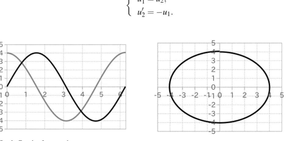
{ u01=u2, (18a)
u02=−u1. (18b)
Fig. 1 Graph ofuk,1anduk,2 Fig. 2 Phase portrait
Figure 1 shows the approximate solutionuk. The horizontal and vertical axes corre- spond to time anduk(t), respectively. Moreover, the black and gray lines showuk,1anduk,2, respectively. Figure 2 is the phase plane ofuk.
In this problem, since n=2 and f(u) = (u2,−u1)T is a linear operator, we adopted L2(J)2as the basic function space for verification, i.e., we choosep=2. The Fr´echet deriva- tive of fat the approximate solutionuk∈Hk1(J)2is given by
f0(uk) = ( 0 1
−1 0 )
.
On the other hand,us∈Hk1(J)2 is defined byus:=Ekξ. Then, the residuals forukandus
are given byre:=−u0k+f(uk)andse:=−u0s+f0(uk)us, respectively. Thereforegξ, which is the right-hand side of the residual equation (6a), is given by
gξ(w) =
( uk,2+us,2+w2−w2−u0k,1−u0s,1
−(uk,1+us,1+w1) +w1−u0k,2−u0s,2 )
=
(re,1+se,1
re,2+se,2
) .
Next, we consider the sufficient condition of (10). From the linearity of the problem, observe that
CL2,L2 sup
ξ∈[ξ]
sup
w∈Wα
gξ(w)
L2(J)2=CL2,L2 sup
ξ∈[ξ]
kre+sekL2(J)2
≤CL2,L2 sup
ξ∈[ξ]
√(kre,1kL2(J)+kse,1kL2(J)
)2
+
(kre,2kL2(J)+kse,2kL2(J)
)2
.
Therefore, if the positive constantαis taken as
α:=CL2,L2
vu ut(
kre,1kL2(J)+sup
ξ∈[ξ]
kse,1kL2(J)
)2
+ (
kre,2kL2(J)+sup
ξ∈[ξ]
kse,2kL2(J)
)2
,
then theFξ-invariance ofWαis satisfied.
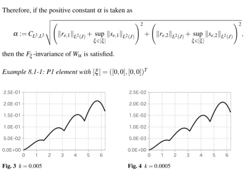
Example 8.1-1: P1 element with[ξ] = ([0,0],[0,0])T
Fig. 3 k=0.005 Fig. 4 k=0.0005
Figure 3 and Fig. 4 show the upper bounds of errors for the approximate solution for the P1 element (Euler method) with uniform step sizek=0.005 andk=0.0005, re- spectively. The horizontal axis is the time and the vertical axis corresponds to the error er:=supu0∈U0|u(t;u0)−uk(t)|. Moreover, the black and gray lines shower,1 ander,2, re- spectively. However, these two lines seem to be almost overlapping in this case.
From the above results, it seems that the errors are increasing in time with order approx- imatelyO(t). These results mean that there is no wrapping effect that causes an exponential increase in the validated region. Moreover, the magnitude of errors in Fig. 4 is approximately
1
10 in Fig. 3. Therefore, we may deduce that our verification algorithm has a convergence orderO(k), which seems to be a reasonable result for using the P1 element (Euler method).
Example 8.1-2: P1 element with[ξ] = ([−0.05,0.05],[−0.05,0.05])T
Fig. 5 k=0.005 Fig. 6 k=0.0005
Figure 5 and Fig. 6 are the verification results from starting with interval initial data. The increase in the validated region still remains approximatelyO(t)even if the initial-value set is fairly big.
Example 8.1-3: P2 element with[ξ] = ([0,0],[0,0])T
Fig. 7 k=0.005 Fig. 8 k=0.0005
Figure 7 and Fig. 8 are the verification results with the P2 element (RK2) and a point initial value. These graphs are also increasing by approximatelyO(t)in time. Moreover, it seems that our verification algorithm has an accuracy ofO(k2), which is also a quite natural result for the P2 element.
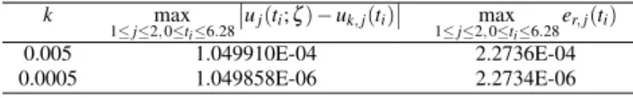
In the present case, since the exact solution of this problem isu(t;ζ) =4(sint,cost)T, we can directly compute the difference betweenuanduk. Table 1 shows the actual errors at nodal points and our verification results. As shown in Table 1, the accuracy of our verifica- tion results is at most twice the exact error.
Table 1 Exact errors and validated range at nodal points
k max
1≤j≤2,0≤ti≤6.28uj(ti;ζ)−uk,j(ti) max
1≤j≤2,0≤ti≤6.28er,j(ti)
0.005 1.049910E-04 2.2736E-04
0.0005 1.049858E-06 2.2734E-06
Example 8.1-4: P2 element with[ξ] = ([−0.05,0.05],[−0.05,0.05])T
Fig. 9 k=0.005 Fig. 10 k=0.0005
Figure 9 and Fig. 10 are the verification results of using the P2 element (RK2) with interval initial data. In this case, it seems that the behavior of the bounds of the validated region is almost independent of the time, for the error bounds are relatively small compared with the width of the interval initial data. The enlargement is at most 10−3for the validated
region in Fig. 9. It is also seen that every graph for this problem repeats the pattern of increasing and decreasing. This phenomenon is due to the fact that the box of the initial- value set leads to a set of closed orbits in the phase space. The length of the diagonal of this box, i.e., 0.05√
2≈0.07071, is the maximum value of Fig. 9.
8.2 Nonlinear problem
In this subsection, we show some verification results for the solutionsu(t;u0) =(
u1(t;u0),u2(t;u0))T
of the following nonlinear ODEs introduced by Yamomoto and Komori [11]:
{ u01=u2, (19a)
u02=u1−u31. (19b)
We now show the results until an ending time of 3.3 so that it is the same length as shown by Yamamoto and Komori [11].
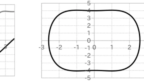
Fig. 11 Graph ofuk,1anduk,2 Fig. 12 Phase portrait
Figure 11 is the graph showing the approximate solutionuk. The black and gray lines correspond touk,1anduk,2, respectively. Figure 12 is the phase plane ofuk.
In this problem, due to the fact thatn=2 andf(u) =(
u2,u1−u31)T
has cubic nonlin- earity, we used the spaceL6(J)2, i.e., we choose p=6. The Fr´echet derivative of f at the approximate solutionuk∈Hk1(J)2is given by
f0(uk) =
( 0 1 1−3u2k,1 0 )
.
We defineus∈Hk1(J)2byus:=Ekξ, as before. Also, the residuals forukandusare defined byre:=−u0k+f(uk)andse:=−u0s+f0(uk)us, respectively. Then, gξ in (6a) is given as follows,
gξ(w) =
( uk,2+us,2+w2−w2−u0k,1−u0s,1
uk,1+us,1+w1−(uk,1+us,1+w1)3−(1−3u2k,1)w1−u0k,2−u0s,2 )
=
( re,1+se,1
−(3uk,1+us,1+w1)(us,1+w1)2+re,2+se,2
) .
Next, we consider the condition of (10). Sincegξ,1is not dependent onw, we have gξ,1(w)
L2(J)≤ kre,1kL2(J)+kse,1kL2(J).
On the other hand, for an arbitraryw∈Wα, we get gξ,2(w)
L2(J)≤ kre,2kL2(J)+kse,2kL2(J)+(
3uk,1+us,1+w1
)(us,1+w1
)2
L2(J). Using the H¨older inequality, the third term of the right-hand side is estimated as
(
3uk,1+us,1+w1
)(us,1+w1
)2
L2(J)≤3uk,1+us,1+w1
L6(J)kus,1+w1k2L6(J)
≤( 3uk,1
L6+kus,1kL6+α)(
kus,1kL6+α)2
.
Therefore, we have
sup ξ∈[ξ]sup
w∈Wα
gξ(w)
L2(J)2= sup ξ∈[ξ] sup
w∈Wα
√gξ,1(w)2
L2(J)+gξ,2(w)2
L2(J)
≤ sup ξ∈[ξ]
√(re,1
L2+se,1
L2
)2
+(re,2
L2+se,2
L2+(
α+us,1
L6+3uk,1
L6
)(α+us,1
L6
)2)2
.
From the above, we obtain a sufficient condition for (10), which leads to a sixth-order alge- braic inequality inα. Therefore, if we find a positive constantαsatisfying this inequality, then it implies theFξ-invariance ofWα.
Example 8.2-1: P1 element with[ξ] = ([0,0],[0,0])T
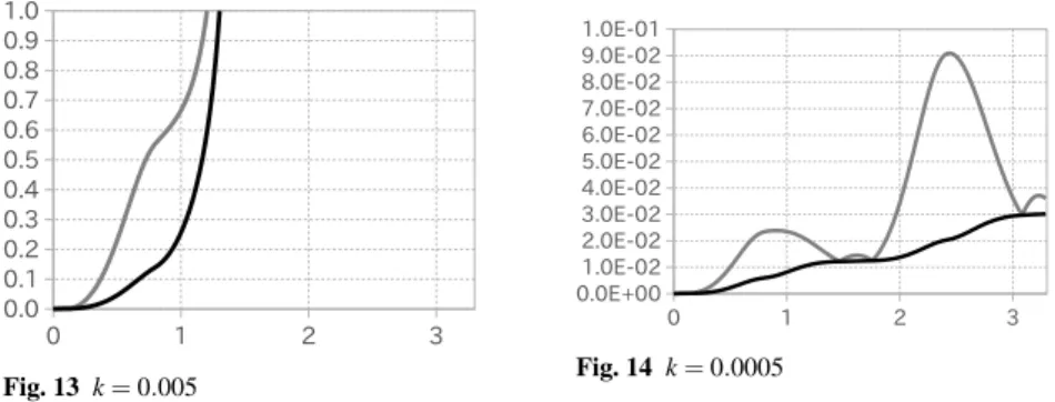
Fig. 13 k=0.005 Fig. 14 k=0.0005
Figure 13 and Fig. 14 show the upper bounds of the errors for the approximate solu- tion for the P1 element (Euler method) with uniform step sizek=0.005 andk=0.0005, respectively. The horizontal and vertical axes correspond to the time and the errorer :=
supu
0∈U0|u(t;u0)−uk(t)|, respectively. Moreover, the black and gray lines shower,1 and er,2, respectively.
As shown in Fig. 13, in the case ofk=0.005, our verification was unsuccessful before T=3.3. On the other hand, by the use of a smaller step size, i.e.,k=0.0005, we successfully verified until the desired time. However, as shown in Fig. 14, the verified accuracy seems to be coarse.
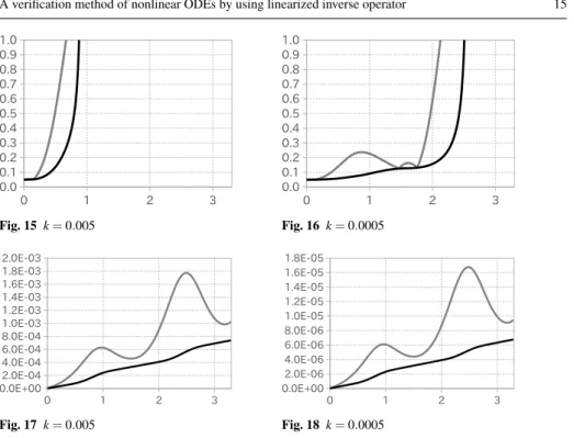
Example 8.2-2: P1 element with[ξ] = ([−0.05,0.05],[−0.05,0.05])T
Figure 15 and Fig. 16 are the verification results with interval initial data. In this case, the verifications were not quickly successful.