RIMS-1747
On the Borel summability of 0-parameter solutions of nonlinear ordinary differential
equations
By
Shingo KAMIMOTO and Tatsuya KOIKE
May 2012
RESEARCH INSTITUTE FOR MATHEMATICAL SCIENCES
On the Borel summability of 0-parameter solutions of nonlinear ordinary differential
equations
Shingo Kamimoto
Research Institute for Mathematical Sciences Kyoto University
Kyoto, 606-8502 JAPAN and
Tatsuya Koike
Department of Mathematics Graduate School of Science
Kobe University Kobe, 657-8501 JAPAN
The research of the authors has been supported in part by GCOE ’Fostering top leaders in mathematics’, Kyoto University and JSPS grants-in-aid No.21740098.
Abstract
In this paper, we announce our recent results on the Borel summability of 0-parameter solutions of second order nonlinear ordinary differential equations with a large parameter. 0-parameter solutions are formal power series solutions with respect to a large parameter, and we es- tablish their Borel summability for a wide class of equations including Painlev´e equations. We also study the singularity structure of a 1- form ω for the Painlev´e equations, which plays an important role in our analysis.
0 Introduction
The main purpose of this article is to announce the results of [KKo]
on the Borel summability of 0-parameter solutions of second order nonlinear ordinary differential equations with a large parameter.
The exact WKB analysis was initiated by A. Voros. He discussed WKB analysis of a Schr¨odinger equation
(0.1)
( d2
dx2 − η2Q(x) )
ψ(x, η) = 0 (η : a large parameter)
using the Borel resummation method ([V]). To employ the exact WKB analysis, it is important to know where the WKB solutions are Borel summable. In [KoS1] and [KoS2], such a problem was studied by considering a formal solution S(x, η) = ηS−1(x) +S0(x) +η−1S1(x) +
· · · of the Riccati equation
(0.2) dS
dx + S2 = η2Q(x)
associated with (0.1). (See also [CDK] and [DLS] for the Borel summa- bility of WKB solutions.)
Following their results we will study in [KKo] the Borel summability
of a formal solution
(0.3) λ(t, η) = λ0(t) + η−1λ1(t) + · · ·
of the second order nonlinear ordinary differential equations of the form
(0.4) d2λ
dt2 = η2P(t, λ)
Q(t, λ) + R1(t, λ,λ)˙ R2(t, λ) ,
where P(t, λ), Q(t, λ), R2(t, λ) ∈ C[t, λ], R1(t, λ,λ)˙ ∈ C[t, λ,λ] and˙ λ˙ = dλ/dt, and P, Q, R1, R2 satisfy some suitable conditions. Typical examples of the above equation (0.4) are Painlev´e equations with a large parameter studied in [KT]. Therefore, following the usage in [KT], we call (0.3) a 0-parameter solution of (0.4) in what follows. In our study, a 1-form
(0.5) ω =
√(∂λP)
(t, λ0(t)) Q(t, λ0(t)) dt
plays a central role when we determine regions in which a 0-parameter solution λ(t, η) is Borel summable: Indeed, the most important condi- tion of the Borel summability of λ(t, η) at t = t0 is that there exists a neighborhood V of t0 such that all of the integral curves of Imω = 0 which pass through V run into singular points of ω of order less than or equal to −1.
This report consists of two sections: In §1, we explain core results of [KKo]. In this report we mainly limit ourselves to the case R1 ≡ 0 in (0.4) to make our arguments clear. In §2, we study the singularity structure ofω for the Painlev´e equations, which is necessary to examine the Borel summability of their 0-parameter solutions.
Acknowledgment.
The authors wish to thank Professor T. Kawai, Professor Y. Takei and their students for the valuable discussions with them and their suggestions.
1 0-parameter solutions and their properties
The main purpose of this section is to give the conditions for the Borel summability of 0-parameter solutions of (0.4). For simplicity, we con- sider the case where R1 ≡ 0, i.e.,
(1.1) d2λ
dt2 = η2P(t, λ) Q(t, λ).
To begin with, let us construct a 0-parameter solution. By multi- plying (1.1) by Q(t, λ), we obtain
(1.2) d2λ
dt2Q(t, λ) = η2P(t, λ).
By substituting (0.3) into (1.2) and comparing both sides degree by degree with respect to η, we find that the coefficients of η2 give
(1.3) P(t, λ0(t)) = 0.
Therefore we choose λ0(t) as a root of (1.3) and fix it in what follows.
Then the lower order terms λ1, λ2,· · · are recursively and uniquely determined when
(1.4) ∂λP(t, λ0(t)) is not identically 0.
Indeed, by comparing the coefficients of η1 of (1.2), we find
(1.5) (
∂λP)
(t, λ0(t))λ1(t) = 0.
Hence we obtain from (1.4) that
(1.6) λ1(t) ≡ 0.
Next, by comparing the coefficients of η0 of (1.2), we find
(1.7) d2λ0
dt2 Q(t, λ0) = (
∂λP)
(t, λ0)λ2(t).
Therefore λ2(t) is given by
(1.8) λ2(t) = Q(t, λ0) (∂λP)
(t, λ0) d2λ0
dt2 .
Then, proceeding the discussion, we can inductively confirm that, by comparing the coefficients of η−n (n = 1,2,· · ·), λn+2(t) are uniquely determined by λ0(t),· · · , λn+1(t) and satisfies
(1.9) λ2k+1(t) ≡ 0 (k = 1,2,· · ·).
In this way, we can uniquely determine a 0-parameter solution of the form
(1.10) λ(t, η) =
∑∞ k=0
η−2kλ2k(t) for each root λ0(t) of (1.3).
Remark 1.1. We immediately find that, if λ2 ≡ 0, then λ2k ≡ 0 (k = 2,3,· · ·). Therefore, in what follows, we assume that λ2 is not identically 0.
Since we cannot expect that the 0-parameter solution (1.10) con- verges, we consider its Borel sum
(1.11) λ0(t) +
∫ ∞
0
e−ηyλ˜B(t, y)dy
with respect to η (see, e.g., [B]). Here ˜λ(t, η) = λ(t, η) −λ0(t) and (1.12) λ˜B(t, y) :=
∑∞ k=1
y2k−1λ2k(t) (2k)!
is the Borel transform of ˜λ(t, η) with respect to η, and the path of integration in (1.11) is the positive real axis as usual.
Our main theorem (Theorem 1.2 below) claims that, under suitable conditions, the integral in (1.11) is well-defined, i.e., ˜λ(t, η) is Borel
summable. Therefore our main concern is to study the analytic prop- erties of ˜λB(t, y) in y-plane. To see how our assumptions naturally appear, let us see the outline of our argument before stating our main theorem.
To study the analytic properties of ˜λB(t, y) we study the Borel tran- soform of (1.2):
(
Q(t, λ0(t)) ∂2
∂t2 − (
∂λP)
(t, λ0(t)) ∂2
∂y2
)λ˜B(t, y) (1.13)
= −d2λ0 dt2
∑
k≥1
1 k!
(∂λkQ(t, λ0))λ˜∗Bk(t, y)
− ∑
k≥1
1 k!
(∂λkQ(t, λ0))∂2λ˜B
∂t2 ∗ λ˜∗Bk(t, y)
+ ∑
k≥2
1 k!
(∂λkP(t, λ0)) ∂2
∂y2
λ˜∗Bk(t, y), where · ∗ · is the convolution operator defined by (1.14) λB ∗ λB =
∫ y 0
λB(t, y − y0)λB(t, y0)dy0 and
(1.15) λ∗Bn =
z }|n { λB ∗ · · · ∗ λB .
We also impose initial conditions which follows from (1.2):
(1.16) λ˜B(t,0) = 0 and ∂λ˜B
∂y (t,0) = λ2(t).
Remark 1.2. We may regard the left-hand side of (1.13) as the principal part in the following sense: when we define the weight of∂/∂t and∂/∂y by 1 and that of · ∗ · by −1, then the left-hand side of (1.13) has the weight 2 and the right-hand side has the weight less than 2.
To simplify left-hand side of (1.13) we employ the Liouville trans- formation, i.e., a coordinate transformation (t, y) 7→ (z, y) defined by
(1.17) z(t) =
∫ t t0
ω, where t0 ∈ C is a fixed point and
(1.18) ω =
√
∂λP(t, λ0(t)) Q(t, λ0(t)) dt.
We assume that ω is holomorphic and does not vanish in the region where we consider. Then, in (z, y)-variable, (1.13) is rewritten as fol- lows:
(1.19) (
∂λP)
(t, λ0) ( ∂2
∂z2 + (dz
dt
)−1d2z dt2
∂
∂z − ∂2
∂y2
)λ˜B(t(z), y).
Further, applying a gauge transformation
(1.20) (
λ2(t))−1λ˜B(t(z), y) =: λbB(z, y), we find that bλB(z, y) satisfies
( ∂2
∂z2 − ∂2
∂y2
)bλB(z, y) (1.21)
= −LbλB(z, y)
− 1
(∂λP)
(t, λ0) 1 λ2
d2λ0 dt2
∑
k≥1
λk2 k!
(∂λkQ(t, λ0))bλ∗Bk(z, y)
− 1
(∂λP)
(t, λ0) (dz
dt
)2∑
k≥1
λk2 k!
(∂λkQ(t, λ0))
× (∂2λbB
∂z2 +LbλB(z, y)
) ∗ bλ∗Bk(z, y)
+ 1
(∂λP)
(t, λ0) 1 λ2
∑
k≥2
λk2 k!
(∂λkP(t, λ0)) ∂2
∂y2bλ∗Bk(z, y),
where
L =
{(dz dt
)−2d2z
dt2 + 2λ−21dλ2 dz
} ∂ (1.22) ∂z
+ (dz
dt
)−2d2z
dt2λ−21dλ2
dz +λ−21d2λ2 dz2 . This bλB(z, y) also satisfies the initial conditions
(1.23) bλB(z,0) = 0 and ∂bλB
∂y (z,0) = 1.
To study a solution of (1.21), we use Proposition 1.1. Let bλB(z, y) satisfy (1.24)
( ∂2
∂z2 − ∂2
∂y2
)bλB(z, y) = Φ(z, y)
and initial conditions
(1.25) λbB(z,0) = 0 and ∂bλB
∂y (z,0) = g(z), where
Φ(z, y) =
∑m
k=1
fk(0)(z)bλ∗Bk(z, y) +
∑m
k=0
fk(1)(z)∂bλB
∂z ∗ bλ∗Bk(z, y) (1.26)
+
∑m
k=1
fk(2)(z)∂2bλB
∂z2 ∗ bλ∗Bk(z, y) +
∑m
k=2
fk(3)(z) ∂2
∂y2λb∗Bk(z, y) and m is a positive integer, and assume that
(1.27) all fk(j)(z) and g(z) are holomorphic and bounded on Er1 = {z ∈ C : |Imz| ≤ r}
for a positive constant r. Then bλB(z, y) is holomorphic on (1.28) Er/22 = {(z, y) ∈ C2 : |Imz| ≤ r/2,|Imy| ≤ r/2}
and satisfies the following estimates for positive constants C1 and C2:
(1.29) |bλB(z, y)| ≤ C1exp[C2|y|].
Indeed, we can rewrite the differential equation to the following in- tegral equation:
(1.30) λbB(z, y) = 1 2
∫ z+y z−y
g(z0)dz0 − 1 2
∫ y 0
∫ z+y−y0 z−y+y0
Φ(z0, y0)dz0dy0, and, employing the iteration method, we can show the above proposi- tion. (See [KKo] for the details.)
Now, our task is to examine the conditions for a 0-parameter solution so that we can apply Proposition 1.1 to it. Our first assumption is (1.31) there exists a neighborhood U of t = t0 and singular points
t = t± of ω of order smaller than −1 such that endpoints of a curve Γˇt are t+ and t− for each point ˇt in U,
where Γtˇ denotes an integral curve of Imω = 0 that passes through a point ˇt. This condition guarantees that z(t) extends to ±∞ along Γtˇ
without encountering any singular point of it. Let Ub denote ∪
ˇt∈U Γˇt. Then we can take r > 0 so that Er1 ⊂ z(Ub) and z(t) is locally biholo- morphic on Ub.
Our second assumption is
(1.32) Ub does not contain t = ∞ in its interior.
(Cf. Remark 1.3 and Remark 1.7.)
Remark 1.3. When we take s = 1/t as a coordinate variable, (1.1) is rewritten as follows:
(1.10) d2λ
ds2 = η2 P(s−1, λ)
s4Q(s−1, λ) − 21 s
dλ ds.
It does not have the form of (1.1). Therefore, when we restrict our equation to the form (1.10), we assume that the discussion is held on C. On the other hand, since P(t, λ) and Q(t, λ) are polynomials, we may regard that (1.10) has the form of (0.4). Hence, as we will mention in Remark 1.7, when we extend the following discussion to (0.4), we do not have to pay special attention to the point ∞ ∈ P1.
By taking the form (1.8) of λ2 into account, it suffices to confirm the holomorphy and the boundedness of the following terms on Ub:
(∂λkP)
(t, λ0)λk2−1 (∂λP)
(t, λ0) and
(∂λkQ)
(t, λ0)λk2
Q(t, λ0) (k ≥ 1).
(1.33)
Indeed, under the assumptions (1.31) and (1.32) (and modifying the gauge transformation (1.20) if necessary), we may assume that the coefficients of L are holomorphic and bounded on Ub.
To guarantee the holomorphy of all terms in (1.33) on Ub, we impose the third assumption:
(1.34) the discriminant DiscP(t) of P(t, λ) and the resultant Res(P,Q)(t) of P(t, λ) and Q(t, λ) do not vanish on Ub.
Note that the condition (1.34) is violated at finitely many points on Ub if DiscP(t) and Res(P,Q)(t) are not identically equal to 0. However, if the terms (1.33) are holomorphic there, then Theorem 1.1 below holds even though (1.34) is violated.
To give the last assumption to ensure the boundedness of the terms (1.33), we prepare some notations. Under the assumption (1.34), by shrinking U if necessary, it suffices to show the boundedness of them at the singular points t±. For simplicity, we assume that t+ ∈ C and λ0(t) behaves as
(1.35) λ0(t) = β+(t − t+)α+ +o(
(t − t+)α+)
with α+ ∈ Q and β+ 6= 0 when t tends to t+. Let F(t, λ) = Fn(t)λn+
· · · + F0(t) ∈ C[t, λ] be a polynomial and assume that Fk(t) (k = 0,1,· · · , n) behave as
(1.36) Fk(t) = Fk(0)(t− t+)νk +o(
(t− t+)νk)
with Fk(0) 6= 0 and νk ∈ Z≥0 = {0,1,2,· · · }. Then, we define an index indtλ+
0(F) (relevant to λ0(t)) by (1.37) indtλ+
0(F) = min
0≤k≤n
{kα+ +νk} and a polynomial DtF+(λ) by
(1.38) DFt+(λ) = ∑
k
Fk(0)λk,
where the sum is taken over k that give the minimum in (1.37), i.e., kα++νk = indtλ+
0(F). In the same way, we can define an index indtλ−
0(F) and a polynomial DtF−(λ) at t = t− for
(1.350) λ0(t) = β−(t− t−)α− + o(
(t −t−)α−) .
We note that the constant β+ in (1.35) (resp., β− in (1.350)) is given by one of the roots of DtP+(λ) = 0 (resp., DPt−(λ) = 0).
Our last assumption is (1.39) D∂t±
λP(β±) 6= 0 and DQt±(β±) 6= 0 hold.
This condition (1.39) entails that the order of ∂λP(
t, λ0(t))
(resp., Q(
t, λ0(t))
) at t = t± coincides with the index indtλ±
0(∂λP) (resp., indtλ±
0(Q)). We also note that the first condition D∂t±
λP(β±) 6= 0 is equivalent to that the leading term β±(t − t±)α± of λ0(t) at t = t± is different from that of the other roots of P(t, λ) = 0. In this sense, if (1.39) holds at t = t±, we call t = t± a nondegenerate singular point.
Further, we can derive the boundedness of the terms (1.33) at t = t± from (1.31) and (1.39).
Remark 1.4. Whent+ = ∞, by takings = t−1 as a coordinate variable, we can define the index indtλ+
0(F) and the polynomial DFt+(λ) in the same manner as above.
Remark 1.5. If the order of the singular points t = t± of ω is strictly less than−1, we can modify the condition (1.39). See [KKo] for details.
Now we state our main theorem:
Theorem 1.1. Let λ0(t) be a root of (1.3) and assume that (1.31), (1.32), (1.34) and (1.39) hold. Then the 0-parameter solution λ(t, η) of (1.1) that has λ0(t) as its initial part is Borel summable on Ub. More precisely, the Borel transform λ˜B(t, y) of λ(t, η) − λ0(t) satisfies the following estimates on Ub × {y ∈ C : |Imy| ≤ r} for positive constants r, C1 and C2:
(1.40) |λ˜B(t, y)| ≤ C1(
|λ2(t)| + 1)
exp[C2|y|].
Remark 1.6. We give a remark here on our results of the Borel summa- bility of 0-parameter solutions in the case when R1 6≡ 0 in (0.4). In this case, λ2(t) is given by
(1.80) λ2(t) = Q(t, λ0) (∂λP)
(t, λ0)
(d2λ0
dt2 − R1(t, λ0,λ˙0) R2(t, λ0)
) .
In addition to the assumptions of Theorem 1.2, if the following terms (1.41) and (1.42) are holomorphic and bounded on Ub, we obtain the same results as Theorem 1.2:
(1.41)
(∂λkR2)
(t, λ0)λk2
R2(t, λ0) and Q(t, λ0) (∂λP)
(t, λ0) d2λ0
dt2
(∂λkR2)
(t, λ0)λk2−1 R2(t, λ0) for k ≥ 0 and
(1.42) Q(t, λ0) (∂λP)
(t, λ0)
(∂λk1∂k˙2
λ R1)
(t, λ0,λ˙0)λ2k1−1λ˙k22 R2(t, λ0)
for {k1, k2 ≥ 0} \ {k1 = k2 = 0}. (See [KKo] for details.)
Remark 1.7. In parallel with Remark 1.3, when we take s = 1/t as a coordinate variable, (0.4) is rewritten as follows:
(0.40) d2λ
ds2 = η2 P(s−1, λ)
s4Q(s−1, λ) − 21 s
dλ
ds + R1(s−1, λ,−s2dλ/ds) s4R2(s−1, λ) . We may regard that (0.40) has the form of (0.4). Therefore, when the terms corresponding to (1.33), (1.41) and (1.42) for (0.40) are holomor- phic and bounded at s = 0, we can extend Theorem 1.1 to the case where Ub contains t = ∞ in its interior.
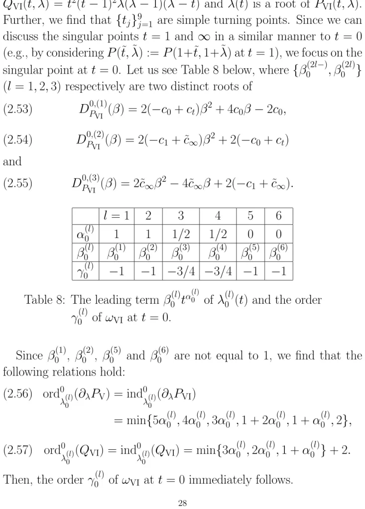
2 Singularity structure of ω for the Painlev´e equations In Section 1, we gave a condition for a 0-parameter solution of (0.4) to be Borel summable. (Cf. Theorem 1.1 and Remark 1.6.) Taking the results into account, we define a turning point and Stokes curves for a 0-parameter solution of (0.4).
Definition 2.1. We call t = t0 a turning point of a 0-parameter solution of (0.4) when the order of a 1-form ω defined by (1.19) at t = t0 is greater than −1, i.e., ω behaves as
(2.1) ω =
{ (C0(t − t0)γ + o((t − t0)γ)) ( dt
C0t−γ−2 + o(t−γ−2)) dt
at t = t0 ∈ C at t = ∞ with C0 6= 0 and γ > −1. Especially, when
∂λP(t0, β0) = 0, (2.2)
∂λ2P(t0, β0) 6= 0, (2.3)
∂tP(t0, β0) 6= 0, (2.4)
Q(t0, β0) 6= 0 (2.5)
hold for a root β0 of P(t0, β0) = 0, we call t = t0 a simple turn- ing point of the corresponding 0-parameter solution. Further, the
integral curves of Im ω = 0 that emanate from turning points are called Stokes curves.
Remark 2.1. In s-variable with s = t−1, the behavior (2.1) of ω at t = ∞ is rewritten as follows:
(2.6) ω = (
−C0sγ + o(sγ))
ds at s = 0.
We remark here that the Borel summability of 0-parameter solutions except on the Stokes curves does not automatically follow. We have to take into account the effect of the lower order term R1/R2 and confirm the nondegeneracy of singular points of ω. In this section, we study the singularity structure of ω for the Painlev´e equations with a large parameter η. (Cf. [KT].)
Remark 2.2. In general, turning points of the Painlev´e equations except for t = 0 of PIII, t = 0 of PV and t = 0,1,∞ of PVI are simple turning points. However, when parameters of the Painlev´e equations satisfy some relations, these simple turning points become “double turning points”. See [T2, Proposition 2.4] for precise conditions.
Example 2.1 (the first Painlev´e equation). We consider the first Painlev´e equation:
(PI) d2λ
dt2 = η2(6λ2 + t).
The 1-form ωI defined by (1.18) for (PI) is given by
(2.7) ωI = √
12λ(t)dt,
and the roots of PI(t, λ) = 6λ2 + t are λ(l)(t) = (−1)l√
−1/6 t1/2 (l = 1,2). Since the discriminant DiscI(t) of PI(t, λ) is
(2.8) DiscI(t) = 144t,
we find that ωI is holomorphic and does not vanish except for t = 0 and ∞.
First, we focus on the behavior of ωI at t = 0. Obviously, t = 0 is a simple turning point of λ(l)(t) (l = 1,2). Then, the index (1.37) for
∂λPI relevant to these λ(l)(t) at t = 0 and the polynomial (1.38) are respectively given by
(2.9) ind0λ(l)(∂λPI) = 1 2 and
(2.10) D0,(l)P
I (β) = 6β2 + 1 = 0 (l = 1,2).
Since DP0,(l)
I (β) has no multiple root, D0,(l)∂
λPI(±√
−1/6) 6= 0, and hence, the order γ0(l) of ωI for λ(l) (l = 1,2) at t = 0 is given by
(2.11) γ0(l) = 1
2ind0
λ(l)(∂λPI) = 1 4.
Second, let us consider the behavior of ωI at t = ∞. Since λ(l)(s) = (−1)l√
−1/6 s−1/2 with s = t−1, the index ind∞
λ(l)(∂λPI) at t = ∞ is given by
(2.12) ind∞λ(l)(∂λPI) = −1
2 (l = 1,2).
Since ωI is represented as
(2.13) ωI = −√
12λ(s)s−2ds
in s-variable, we find the order γ∞(l) of ωI for λ(l) (l = 1,2) at t = ∞ is given by
(2.14) γ∞(l) = 1
2ind∞λ(l)(∂λPI) − 2 = −9
4 (l = 1,2).
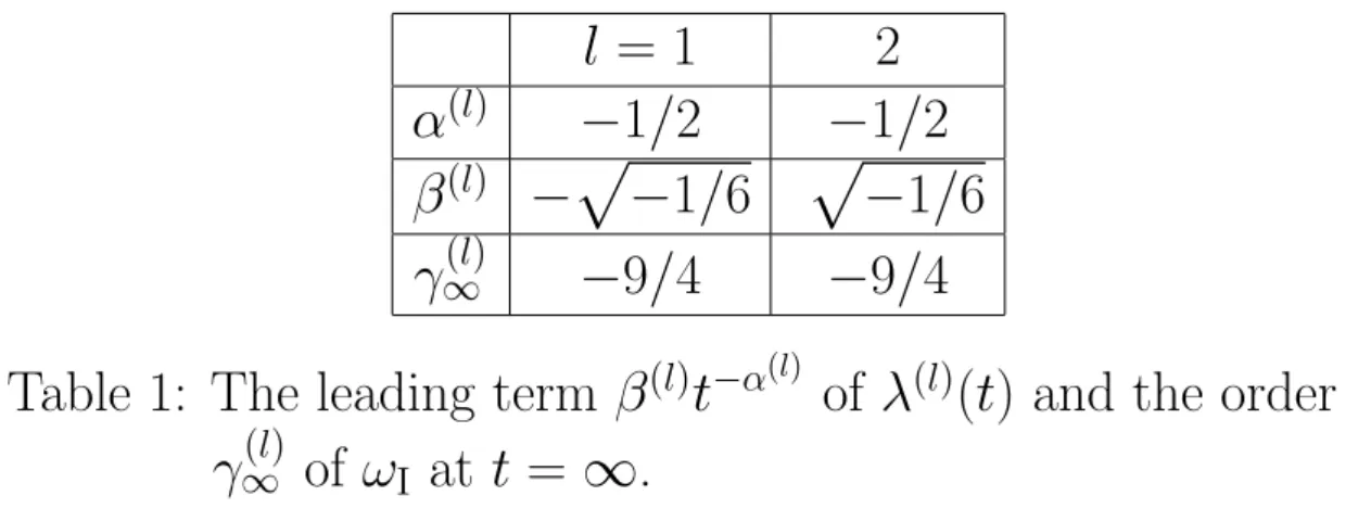
l = 1 2 α(l) −1/2 −1/2 β(l) −√
−1/6 √
−1/6 γ∞(l) −9/4 −9/4
Table 1: The leading term β(l)t−α(l) of λ(l)(t) and the order γ∞(l) of ωI at t = ∞.
Remark 2.3. We find that the above discussion indicates the Borel summability of 0-parameter solutions of (PI) except on the Stokes curves emanating from t = 0, and hence, we can take the Borel sum of them. On the other hand, as is discussed in [T1], t = 0 actually behaves as a turning point and 0-parameter solutions of (PI) are not Borel summable on these Stokes curves. Hence, when we consider the analytic continuation of the Borel sum of a 0-parameter solution across a Stokes curve, Stokes phenomena occur, and a so-called “1-parameter solution” appears. We can also show the generalized Borel summability of it. See [K] for the details. Here, we mention that a similar kind of formal solutions called “transseries solutions” are studied in [C], which are the formal exponential series solutions at an irregular singular point of nonlinear ordinary differential equations. Further, the generalized Borel summability of transseries solutions is discussed there.
Example 2.2 (the second Painlev´e equation). Next, we consider the second Painlev´e equation
(PII) d2λ
dt2 = η2(2λ3 + tλ+ c).
We discuss on the singular points of
(2.15) ωII = √
6λ2(t) + t dt
with a root λ(t) of PII(t, λ) = 2λ3+tλ+c. The discriminant DiscII(t) of PII(t, λ) is given by
(2.16) DiscII(t) = 8(2t3 + 27c2).
Therefore, when c 6= 0, DiscII(t) = 0 has three distinct roots, i.e., t = tj := 3θj(c2/2)1/3 (j = 0,1,2) with θ = exp[2π√
−1/3]. In what follows, we assume that c 6= 0. We examine the behavior of the roots of PII(t, λ) = 0 and ωII for the roots at t = tj. We first note that three roots of PII(t, λ) = 0 behave as λ(l)j (t) = βj(l) + o(1) (l = 1,2,3) at t = tj, where {βj(l)}3l=1 are the roots of
(2.17) DPtj,(l)
II (β) = 2β3 +tjβ +c (l = 1,2,3).
Since DiscII(tj) = 0, two of them coincide. Let βj(1) = βj(2) be such roots. Then, we immediately find that t = tj is a simple turning point of λ(l)j (t) (l = 1,2). Since ∂βDPtj,(1)
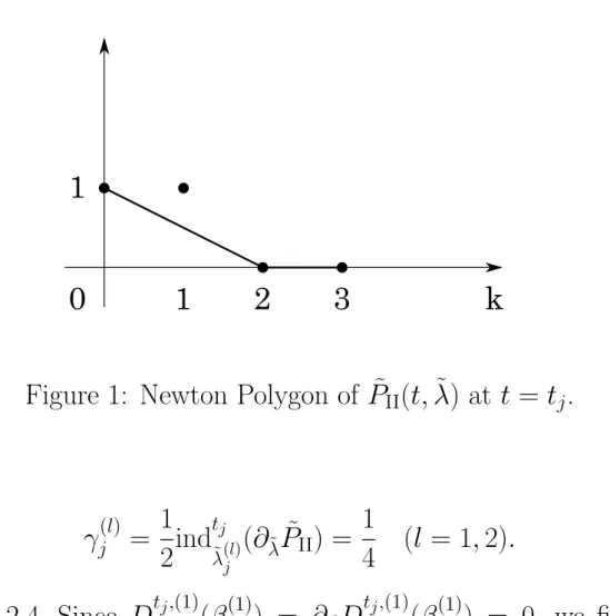
II (βj(1)) = 6(βj(1))2 + tj = 0, the Newton polygon of ˜PII(t,λ) :=˜ PII(t, βj(1) + ˜λ) = 2˜λ3+ 6βj(1)λ˜2+ (t− tj)˜λ+βj(1)(t−tj) at t = tj is given by Figure 1 below. Therefore, two of the roots ˜λ(1)j (t) and ˜λ(2)j (t) of ˜PII(t,λ) behave as˜
(2.18) λ˜(l)j (t) = ˜βj(l)(t − tj)1/2 +o((t − tj)1/2) (l = 1,2), where ˜βj(l) are the two distinct roots of
(2.19) Dt˜j,(l)
PII ( ˜β) = 6 ˜β2 + 1 = 0 (l = 1,2), and hence,
(2.20) indtj
λ˜(l)j (∂˜λP˜II) = min {
1, 1
2,2· 1 2
}
= 1
2 (l = 1,2).
Therefore, the order γj(l) of ωII for λ(l)j (t) (l = 1,2) at t = tj is given
Figure 1: Newton Polygon of ˜PII(t,λ) at˜ t = tj. by
(2.21) γj(l) = 1 2indtj
λ˜(l)j (∂λ˜P˜II) = 1
4 (l = 1,2).
Remark 2.4. Since D∂tj,(1)
λPII(βj(1)) = ∂βDPtj,(1)
II (βj(1)) = 0, we find that t = tj (j = 1,2,3) are degenerate singular points, and hence,
(2.22) γj(l) > 1 2indtj
λ(1)j (∂λPII) = 0.
However, by considering ˜λ(l)j (t) (l = 1,2) and ˜PII(t,λ) instead of˜ λ(l)j (t) (l = 1,2) and PII(t, λ), we can reduce these singular points to nonde- generate ones as above. Then, we can measure the order γj(l) by the index indtj
λ˜(l)j (∂λ˜P˜II) as (2.21).
On the other hand, since ∂βDtPj,(3)
II (βj(3)) 6= 0, we find that the other root λ(3)j (t) is holomorphic at t = tj, and hence, ωII for λ(3)j (t) is also
holomorphic and does not vanish there.
Now, let us focus on the singular points of ωII at t = ∞. We find that three roots of ˜PII(t,λ) behave as Table 2 below.˜
l = 1 2 3
α(l)∞ 1 −1/2 −1/2 β∞(l) −c √
−1/2 −√
−1/2 γ∞(l) −5/2 −5/2 −5/2
Table 2: The leading term β∞(l)t−α(l)∞ of λ(l)∞(t) and the order γ∞(l) of ωII at t = ∞.
Table 2 indicates that D∞P ,(l)
II (β) (l = 1,2,3) has no multiple root.
Hence, the order ord∞
λ(l)∞(∂λPII) of ∂λPII(t, λ(l)∞(t)) at t = ∞ is given by (2.23) ord∞
λ(l)∞(∂λPII) = ind∞˜
λ(l)∞(∂λPII) = min{2α(l)∞,−1}.
Therefore, we find that the order γ∞(1) of ωII for λ(1)∞(t) at t = ∞ is given by
(2.24) γ∞(1) = 1
2ind∞
λ(1)∞(∂λPII) − 2 = −5 2.
On the other hand, the order γ∞(l) of ωII for the other roots is given by (2.25) γ∞(l) = 1
2ind∞
λ(l)∞(∂λPII) − 2 = −5
2 (l = 2,3).
Example 2.3 (the third Painlev´e equation). Let us consider the third Painlev´e equation
(PIII) d2λ dt2 = 1
λ (dλ
dt )2
− 1 t
dλ
dt + 8η2 [
2c∞λ3 + c0∞
t λ2 − c00
t − 2c0 λ
] .
In what follows, we assume that c∞, c0∞, c00 and c0 are not equal to 0.
Let ωIII be a 1-form defined by (2.26) ωIII =
√ 8(
8c∞tλ3(t) + 3c0∞λ2(t) − c00)
tλ(t) dt
with a root λ(t) of PIII(t, λ) = 8(
2c∞tλ4 +c0∞λ3−c00λ−2c0t)
. Since the discriminant DiscIII(t) of PIII(t, λ) and the resultant ResIII(t) of PIII(t, λ) and QIII(t, λ) = tλ are respectively given by
DiscIII(t) =N1c∞t(
(c0∞)3(c00)3 − (27c∞2 (c00)4 + 27(c0∞)4c20 (2.27)
− 6c∞(c0∞)2(c00)2c0)t2 + 768c2∞c0∞c00c20t4 − 4096c3∞c30t6) and
(2.28) ResIII(t) = N2c0t5
with some integersN1 andN2, ωIII may have six singular points {tj}6j=1
except fort = 0 and∞ in general. Indeed, the discriminant of DiscIII(t) is written as
(2.29) N c25∞(c0∞)9(c00)9c120 (
c∞(c00)2 − (c0∞)2c0)8(
c∞(c00)2 + (c0∞)2c0)4
with some integer N, and hence, DiscIII(t) has seven distinct roots when it does not vanish. Since DiscIII(tj) = 0 (j = 1,2,· · · ,6), two of the roots βj(1) and βj(2) of PIII(tj, β) = 0 coincide. Then, we find that t = tj are simple turning points and that two of the roots ˜λ(1)j (t) and λ˜(2)j (t) of ˜PIII(t,λ) :=˜ PIII(t, βj(1) + ˜λ) behave as
(2.30) λ˜(l)j (t) = ˜βj(l)(t −tj)1/2 +o((t − tj)1/2), where ˜βj(l) are the two distinct roots of
(2.31) Dt˜j,(l)
PIII ( ˜β) = 1
2∂λ2PIII(tj, βj(1)) ˜β2 +∂tPIII(tj, βj(1)) = 0 (l = 1,2).
Indeed, ∂λ2PIII(tj, βj(1)) and ∂tPIII(tj, βj(1)) do not vanish when c∞(c00)2
−(c0∞)2c0 6= 0, and hence, we can read the behavior of ˜λ(l)j (t) (l = 1,2) at t = tj from Figure 2.
Figure 2: Newton Polygon of ˜PIII(t,λ) at˜ t = tj.
Since ResIII(tj) 6= 0 (j = 1,2,· · · ,6), the order of QIII(t, λ(l)j (t)) (l = 1,2,3,4) at t = tj coincide with indtj
λ(l)j (QIII) = 0. Therefore, the order γj(l) of ωIII for λ(l)j (t) (l = 1,2) at t = tj is given by
(2.32) γj(l) = 1 2
(indtj
λ˜(l)j (∂λ˜P˜III) − indtj
λ(l)j (QIII))
= 1
4 (l = 1,2).
On the other hand, we immediately see that the other roots λ(l)j (t) (l = 3,4) are holomorphic at t = tj and ωIII for these roots is also holomorphic and does not vanish there when c∞(c00)2 + (c0∞)2c0 6= 0.
Otherwise, one more multiple root βj(3)(= βj(4)) appears. However, applying the same reasoning as above to the pair λ(3)j (t) and λ(4)j (t),