RIMS-1833
Randomized Strategies for Cardinality Robustness in the Knapsack Problem
By
Yusuke KOBAYASHI and Kenjiro TAKAZAWA
August 2015
R ESEARCH I NSTITUTE FOR M ATHEMATICAL S CIENCES
Randomized Strategies for Cardinality Robustness in the Knapsack Problem
Yusuke Kobayashi∗ Kenjiro Takazawa† August 5, 2015
Abstract
We consider the following zero-sum game related to the knapsack problem. Given an instance of the knapsack problem, Alice chooses a knapsack solution and Bob chooses a cardinality k with knowing Alice’s solution. Then, Alice obtains a payoff equal to the ratio of the profit of the best k items in her solution to that of the best solution of size at most k. Forα > 0, a knapsack solution is called α-robust if it guarantees payoff α. If Alice adopts a deterministic strategy, the objective of Alice is to find a max-robust knapsack solution. By applying the argument in Kakimura and Makino (2013) for robustness in general independence systems, a 1/√µ-robust solution exists and is found in polynomial time, whereµis the exchangeability of the independence system.
In the present paper, we address randomized strategies for this zero-sum game. Random- ized strategies in robust independence systems are introduced by Matuschke, Skutella, and Soto (2015) and they presented a randomized strategy with 1/ln(4)-robustness for a certain class of independence systems. The knapsack problem, however, does not belong to this class.
We first establish the intractability of the knapsack problem by showing an instance such that the robustness of an arbitrary randomized strategy is O(log logµ/logµ) and O(log logρ/logρ), where ρ is the ratio of the size of a maximum feasible set to that of minimum infeasible set minus one. We then exhibit the power of randomness by designing two randomized strategies with robustness Ω(1/logµ) and Ω(1/logρ), which substantially improve upon that of deter- ministic strategies and almost attain the above upper bounds. It is also noteworthy that our strategy applies to not only the knapsack problem but also independence systems for which an (approximately) optimal solution under a cardinality constraint is computable.
Keywords: Robust independence system, Randomized strategy, Knapsack problem, Exchangeability
1 Introduction
1.1 Cardinality robustness in independence systems
Cardinality robustnessin independence systems is introduced by Hassin and Rubinstein [3], defined as follows. Let (E,F) be an independence system. That is,E is a finite set of items and F ⊆2E
∗University of Tsukuba. Supported by JST, ERATO, Kawarabayashi Project, by JSPS KAKENHI Grant Number 24700004, and by MEXT KAKENHI Grant Number 24106002. E-mail: [email protected]
†Research Institute for Mathematical Sciences, Kyoto University. Partially supported by JSPS KAKENHI Grant Numbers 25280004 and 26280001. E-mail: [email protected]
is the feasible set family satisfying that ∅ ∈ F and X ⊆Y ∈ F implies X ∈ F. A feasible set is often referred to as a solution. Letpe∈R+ represent the profit of item e∈E, and let OPTk ⊆E be a feasible set maximizing its profit among those of size at most k. That is, OPTk satisfies that OPTk∈ F,|OPTk| ≤k, and p(OPTk) = max{p(X)|X∈ F,|X| ≤k}, where the profit p(X) of a feasible setX is defined byp(X) :=∑
e∈Xpe. ForX∈ F, letX(k) denote a subset ofX satisfying that |X(k)| ≤k and p(X(k)) = max{p(X′) | X′ ⊆ X,|X′| ≤ k}. Intuitively, X(k) consists of k p-highest items in X. Forα >0, a feasible setX ∈ F is called α-robust ifp(X(k))≥α·p(OPTk) for an arbitrary positive integerk.
Our problem is to find a feasible set with large robustness. This is described as the following zero-sum game.
Alice chooses a feasible setX∈ F, and Bob chooses a cardinalitykwith knowing Alice’s set. Then, Alice obtains a payoff p(X(k))/p(OPTk).
In this zero-sum game, the objective of Alice is to find a feasible set with maximum robustness.
It is not difficult to see that, ifF is the independent set family of a matroid onE, then a greedy solution is 1-robust. More generally, Hassin and Rubinstein [3] proved that a greedy solution is r(F)-robust, wherer(F) is therank quotient of (E,F) [4, 7].
Ap2-optimal solution, i.e., a feasible setX∈ F maximizing∑
e∈Xp2e, often has larger robustness than a greedy solution. Hassin and Rubinstein [3] showed that a p2-optimal matching is 1/√
2- robust, and there exist graphs not containing an α-robust matching for an arbitrary α > 1/√
2.
Fujita, Kobayashi, and Makino [2] discussed the case whereF is defined by matroid intersection, i.e., common independent sets of two matroids onE, and proved that ap2-optimal common independent set is 1/√
2-robust. It is also shown in [2] that determining whether a graph has an α-robust matching is NP-hard for an arbitrary α > 1/√
2. Analysis for general independence systems is due to Kakimura and Makino [5], who proved that a p2-optimal feasible set is a 1/√
µ(F)-robust solution, whereµ(F), theexchangeability of (E,F), is defined as the minimum integerµsatisfying that
∀X, Y ∈ F, ∀e∈Y −X, ∃Z ⊆X−Y s.t.|Z| ≤µ, (X−Z)∪ {e} ∈ F. (1) In [5], it is also shown that the above robustness is tight in the sense that for an arbitrary positive integerµ, there exists an independence system (E,F) such thatµ(F) =µand noα-robust solution exists for arbitrary α >1/√
µ.
Kakimura, Makino, and Seimi [6] focused on the case where (E,F) is defined by an instance of the knapsack problem. An instance (E, p, w, C) of the knapsack problem consists of the set E of items, the profit vector p ∈ RE+, the weight vector w ∈ RE+, and the capacity C ∈ R+. A subsetX⊆E is feasible if its weightw(X) :=∑
e∈Xweis at most the capacity, i.e.,F ={X ⊆E| w(X) ≤C}. Kakimura, Makino, and Seimi [6] proved that the problem of computing a knapsack solution with the maximum robustness is weakly NP-hard, and also presented an FPTAS for this problem.
1.2 Randomized strategies
The above results correspond to deterministic strategies (or pure strategies) of the zero-sum game.
Matuschke, Skutella, and Soto [8] introduced randomized strategies (or mixed strategies) for the robust independence systems. In this setting, Alice calls a probability distribution on the feasible
sets, and Bob chooses an integer k with knowing the distribution of Alice. The robustness of Alice’s strategy is defined by the expected payoff. That is, if Alice chooses a distribution in which a solution Xi has probabilityλi, then the robustness of this strategy is
mink
E[p(Xi(k))]
p(OPTk) = min
k
∑
iλip(Xi(k)) p(OPTk) .
For the robust matching case, Matuschke, Skutella, and Soto [8] presented a randomized strategy with robustness 1/ln(4), a significant improvement upon the robustness 1/√
2 of the deterministic strategy. They further showed that this strategy applies to bit-concave independence systems, which are defined as follows.
If pe = 2le for eache∈E with le ∈Z (i.e.,p is a bit-function), then a greedy solution is 1-robust. Equivalently, for an arbitrary bit-function p, it holds that 2p(OPTk+1) ≥ p(OPTk) +p(OPTk+2) for all k∈Z>0 (bit-concavity).
Examples of bit-concave independence systems include matroid intersection, b-matchings, strongly base orderable matchoids, strongly base orderable matroid parity systems.
1.3 Our results
We address randomized strategies for the robust independence systems defined by an instance of the knapsack problem. It is not difficult to see that those independence systems are not necessarily bit-concave.
We provide upper and lower bounds for the robustness in terms of the exchangeability µ(F) and a new parameterρ(F), defined by
ρ(F) := amax
amin
, amax:= max{|X| |X∈ F}, amin:= min{|X| |X̸∈ F} −1. (2) We remark that the parameters µ(F) and ρ(F) represent the intractability of the independence system (E,F). Clearlyµ(F)≥1 andρ(F)≥1,µ(F) = 1 holds if and only ifF is the independent set family of a matroid, and ρ(F) = 1 holds if and only if F is the independent set family of a uniform matroid. If F is defined by the matchings in a graph, then µ(F) ≤2. For the problem of finding a feasible setX maximizing p(X), the greedy algorithm attains 1/µ(F)-approximation [9].
A greedy solution also yields 1/ρ(F)-approximation as well (see Proposition 2). We also note that ρ is a parameter whose definition is similar to 1/r(F). Thus, roughly speaking, the larger µ(F) or ρ(F) becomes, the harder optimization over (E,F) becomes.
We first establish the intractability of the robust knapsack problem by showing a family of instances which do not admit a randomized strategy with constant robustness. Indeed, for those in- stances, we prove that the robustness of an arbitrary randomized strategy is O(log logµ(F)/logµ(F)) and O(log logρ(F)/logρ(F)).
We then exhibit the power of randomness by designing two randomized strategies with ro- bustness Ω(1/logµ(F)) and Ω(1/logρ(F)). These lower bounds substantially improve upon that of deterministic strategies, and almost attain the above upper bounds. Roughly speaking, the Ω(1/logρ(F))-robust strategy is a uniform distribution of the optimal solutions under different cardinality constraints, which are efficiently computed by an FPTAS [1]. In the Ω(1/logµ(F))- robust strategy, we modify the Ω(1/logρ(F))-robust strategy so that some items in the optimal solution are always chosen, which helps attaining good robustness whenµ(F) is small.
Furthermore, we extend the aforementioned results to general independence systems. We show that the Ω(1/logρ(F))-robust strategy is applied to general independence systems. We also provide upper bounds O(1/logρ(F)) and O(1/logµ(F)) on robustness, which proves the tightness of our Ω(1/logρ(F))-robust strategy.
We also point out that an independence system defined by an instance (E, p, w, C) of the knapsack problem is an example of an independence system which is bit-concave but not concave, when all items have unit densities, i.e., pe/we is identical. This provides an answer to a question posed by [8].
1.4 Organization of the paper
The rest of this paper is organized as follows. In Section 2, we show an instance of the knap- sack problem for which no randomized strategy attains constant robustness, and provide upper bounds O(log logµ(F)/logµ(F)) and O(log logρ(F)/logρ(F)) on robustness. Our randomized strategies with robustness Ω(1/logµ(F)) and Ω(1/logρ(F)) appear in Section 3. Bit-concavity in the unit density case is also discussed in this section. In Section 4, we discuss general independence systems. Section 5 concludes this paper with a few remarks.
2 Upper Bounds on Robustness
As we described in Section 1.2, there exists a randomized strategy with robustness at least 1/ln(4) for bit-concave independence systems [8]. In this section, we show that there exists an instance of the knapsack problem for which no randomized strategy can achieve a constant robustness.
Theorem 1. For an arbitrary constant κ > 0, there exists an instance of the knapsack problem such that the robustness of an arbitrary randomized strategy is less than κ.
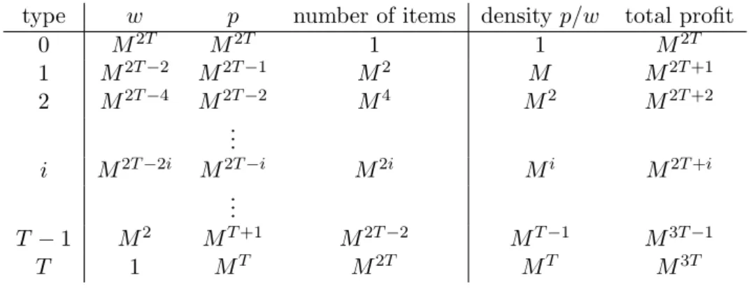
Proof. For a given constantκ >0, letM andT be integers larger than 3/κ. Consider the following instance of the knapsack problem (see Table 1).
• There are T+ 1 types of items, say type 0, type 1, . . . , typeT.
• For eachi= 0,1, . . . , T, there areM2i items of typei, and the weight and profit of each item of typeiare M2T−2i and M2T−i, respectively.
• The capacity is C=M2T.
Observe that the total weight of the items of type i is equal to C for each i. Since the den- sitype/weof an itemeof typeibecomes larger for largei, it is better to choose items of typeiwith large i under a soft cardinality constraint. However, the profit of a single item of type iis small for largei, and hence it is better to choose items with smalliunder a hard cardinality constraint.
For this instance, we show that the robustness of an arbitrary randomized strategy is less than κ.
Let ∆ ⊆ RT++1 be the set of all vectors δ = (δ0, δ1, . . . , δT) ∈ RT++1 such that δiM2i is an integer for i = 0,1, . . . , T and ∑
iδi ≤1. For δ ∈ ∆, let Xδ ⊆ E denote the feasible solution of the knapsack instance that contains δiM2i items of type ifori= 0,1, . . . , T. Note that ∑
iδi ≤1 corresponds to the capacity constraint and there is a one-to-one correspondence between ∆ and the set of all feasible solutions.
Table 1: An instance denying a constant robustness. The capacity isC =M2T. type w p number of items densityp/w total profit
0 M2T M2T 1 1 M2T
1 M2T−2 M2T−1 M2 M M2T+1
2 M2T−4 M2T−2 M4 M2 M2T+2
...
i M2T−2i M2T−i M2i Mi M2T+i ...
T−1 M2 MT+1 M2T−2 MT−1 M3T−1
T 1 MT M2T MT M3T
Since the set of all items of type iis a feasible solution, we have that p(OPTM2i)≥M2T+i for each i= 0,1, . . . , T. For eachδ ∈∆ and for each i∈ {0,1, . . . , T}, it holds that
p(Xδ(M2i))≤
i−1
∑
j=0
δjM2j·M2T−j +δiM2i·M2T−i+M2i·M2T−i−1,
where the last term bounds the total weight of the items of types i+ 1, i+ 2, . . . , T in Xδ(M2i), because each weight is at mostM2T−i−1 and the number of items is at most M2i. The right hand side of this inequality is bounded by
∑i−1
j=0
δj
M2T+i−1+δiM2T+i+M2T+i−1≤δiM2T+i+ 2M2T+i−1,
which shows that
p(Xδ(M2i))≤ (
δi+ 2 M
)
·p(OPTM2i) (i= 0,1, . . . , T).
Hence, for a randomized strategy choosing Xδ with probabilityλδ, it holds that
∑
δ∈∆
λδp(Xδ(M2i))≤ (∑
δ∈∆
λδδi+ 2 M
)
·p(OPTM2i) (i= 0,1, . . . , T),
which implies that the robustness of this strategy is at most mini{∑
δ∈∆λδδi+ 2/M}. On the other hand, since
∑T i=0
(∑
δ∈∆
λδδi
)
=∑
δ∈∆
( λδ
∑T i=0
δi
)
≤∑
δ∈∆
λδ= 1, it follows that mini{∑
δ∈∆λδδi} ≤1/(T+ 1). Therefore, the robustness is at most T+11 +M2 , which is smaller thanκ.
Since Theorem 1 shows that no randomized strategy can achieve a constant robustness, a reasonable objective is to achieve a good robustness in terms of some parameters. We can see that the difficulty of the above instance comes from the huge gap between the weights of light items and heavy items, which makesµ(F) andρ(F) larger. Recall thatµ(F) andρ(F) are defined in (1) and (2), respectively.
In what follows, we takeµ(F) andρ(F) as parameters. We first show that the greedy algorithm attains 1/ρ(F)-approximation for finding a feasible set X maximizing p(X), as well as 1/µ(F)- approximation [9]. Here, the greedy algorithm means adding an element with highest profit to the solution as long as it is feasible. This suggests that µ(F) and ρ(F) represent the intractability of the independence system (E,F).
Proposition 2. Let (E,F) be an independence system and p ∈ RE+ be a profit vector. For the problem of finding a feasible set X ∈ F maximizing p(X), the greedy algorithm finds a 1/ρ(F)- approximate solution.
Proof. LetY and OPT be the output of the greedy algorithm and an optimal solution, respectively.
By the definition of amin,Y containsamin highest profit elements in E, that is, E(amin)⊆Y. Let p0 := min{pe |e∈E(amin)}. Since pe′ ≤ p0 for each e′ ∈ OPT−OPT(amin) and |OPT| ≤amax, we have
p(OPT) =p(OPT(amin)) +p(OPT−OPT(amin))
≤p(E(amin)) + (|OPT| −amin)p0
≤p(E(amin)) + (amax−amin)·p(E(amin)) amin
= 1
ρ(F) ·p(E(amin))
≤ 1
ρ(F) ·p(Y),
which shows thatY is a 1/ρ(F)-approximate solution.
The proof of Theorem 1 shows that, for the instance in Table 1, the robustness of an arbitrary randomized strategy is O(log logρ(F)/logρ(F)) and O(log logµ(F)/logµ(F)).
Theorem 3. There exists an independence system (E,F) defined by an instance of the knapsack problem such that the robustness of an arbitrary randomized strategy is O(log logµ(F)/logµ(F)) and O(log logρ(F)/logρ(F)).
Proof. Let T = M in Table 1. Then, µ(F) = ρ(F) = M2M and the robustness of an arbitrary randomized strategy is at most 3/M. Since logM2M = Θ(MlogM) and log logM2M = Θ(logM), we obtain the theorem.
We close this section with remarking that ratio µ(F)/ρ(F) can be arbitrarily large and small.
To see this, consider an instance of the knapsack problem in which C = 2M, there is one item of weight M, and there are 2M items of weight 1. In this instance, µ(F) = M and ρ(F) = 2M/(M+ 1)<2, which shows thatµ(F)/ρ(F) can be arbitrarily large. Also, consider an instance in whichC= 2M−1, there are two items of weightM, and there areM items of weight 1. In this instance,µ(F) = 1 and ρ(F) =M, showing thatµ(F)/ρ(F) can be arbitrarily small.
3 Randomized Strategies
We have already seen that the robustness of an arbitrary randomized strategy is O(log logµ(F)/logµ(F)) and O(log logρ(F)/logρ(F)). This section is devoted to presenting positive results, randomized strategies with robustness Ω(1/logρ(F)) and Ω(1/logµ(F)) in Sections 3.1 and 3.2, respectively.
Theorem 3 suggests that these results are almost tight, and the latter robustness substantially im- proves upon the robustness 1/√
µ(F) of a deterministic strategy in [5]. We also show in Section 3.3 that 1/ln(4)-robust strategy in [8] works for the case when all items have unit densities, i.e.,pe/we is identical.
3.1 An Ω(1/logρ(F))-robust strategy
In this subsection, we present a randomized strategy with robustness Ω(1/logρ(F)). Recall that ρ(F) is defined in (2).
Theorem 4. For an arbitrary independence system (E,F) defined by an instance of the knapsack problem, there is a randomized strategy with robustness Ω(1/logρ(F)).
Proof. Let (E,F) be defined by an instance (E, p, w, C) of the knapsack problem and let m =
⌈logρ⌉. Recall that, for eachk, OPTk is an optimal solution of (E, p, w, C) subject to|OPTk| ≤k.
Our randomized strategy is described as follows.
Strategy 1. Choose Xi:= OPT2iamin with probability 1/(m+ 1) for each i∈ {0,1, . . . , m}. We now show that the robustness of Strategy 1 is at least 1/(m+ 1) = Ω(1/logρ(F)).
• For an integerkwithamin≤k <2mamin, letjbe an integer satisfying 2jamin ≤k <2j+1amin. Then, we have that
p(Xj(k)) =p(
OPT2jamin)
≥p(OPTk(2jamin))≥ 2jamin
k ·p(OPTk)≥ 1
2 ·p(OPTk).
We also have that
p(Xj+1(k))≥ k
2j+1amin ·p(Xj+1)≥ k
2j+1amin ·p(OPTk)≥ 1
2 ·p(OPTk).
Thus,
E[p(X(k))] = 1 m+ 1
∑m i=0
p(Xi(k))≥ 1
m+ 1·(p(Xj) +p(Xj+1(k)))≥ 1
m+ 1·p(OPTk).
• For an integerk≤amin, we havep(X0(k)) =p(OPTk), sinceX0 = OPTamin is the set ofamin
highest profit elements inE. Thus, E[p(X(k))]≥ 1
m+ 1·p(X0(k)) = 1
m+ 1·p(OPTk).
• For an integerk≥2mamin, it holds thatp(OPTk) =p(Xm) =p(Xm(k)). Thus, E[p(X(k))]≥ 1
m+ 1·p(Xm(k)) = 1
m+ 1·p(OPTk).
Therefore, we conclude that the robustness of Strategy 1 is at least 1/(m+ 1).
We remark that computing OPT2iaminis NP-hard. In order to obtain the strategy in polynomial time, we efficiently compute a solution Xi approximating OPT2iamin for each ivia an FPTAS for the knapsack problem with a cardinality constraint [1].
Corollary 5. For an arbitrary independence system (E,F)defined by an instance of the knapsack problem, an Ω(1/logρ(F))-robust randomized strategy is obtained in polynomial time.
We also note that we can slightly improve the bound by following the proof of Theorem 4. Let a∗max be the size of a minimum optimal solution of the knapsack problem. Then, we can replace amax with a∗max in the proof to obtain an Ω(1/log(a∗max/amin))-robust strategy, which is slightly better than Ω(1/logρ(F)).
3.2 An Ω(1/logµ(F))-robust strategy
In this subsection, we present an Ω(1/logµ(F))-robust randomized strategy, where µ(F) is the exchangeability of the independence system (E,F). Note that, for the case where only deterministic strategies are allowed, Kakimura and Makino [5] showed the existence of 1/√
µ(F)-robust solution.
That is, we improve this ratio to Ω(1/logµ(F)) by allowing randomized strategies, to prove the power of randomness in the robust knapsack problem. Our strategy is based on the ideas in Section 3.1, but we need extra work for this case.
Theorem 6. For an arbitrary independence system (E,F) defined by an instance of the knapsack problem, there is a randomized strategy with robustness Ω(1/logµ(F)).
Proof. Let (E,F) be defined by an instance (E, p, w, C) of the knapsack problem. In this proof we often abbreviateµ(F) asµ. We may assume that the weight of each element is at most C and w(E)> C. Let Y ⊆E be an optimal solution of this problem, and let Z ⊆ E be the set ofamin heaviest elements in E. Note that w(Z)≤C by the definition ofamin.
Since |Y|/|Z| ≥ a∗max/amin, we can apply Strategy 1 when |Y|/|Z| ≤ µ (see a remark after Corollary 5). We now address the case when |Y|/|Z| is much larger. In such a case, we choose many light elements in Y in advance (with ignoring their profit), which is our main idea in the proof. Let Y0 be the subset of Y that maximizes |Y0|subject to w(Y0) ≤C−w(Z). That is, Y0
is obtained by taking light elements inY greedily as long asw(Y0)≤C−w(Z). Now we have the following lemma.
Lemma 7. It holds that µ|Z| ≥ |Y −Y0|.
Proof of Lemma 7. We first show the existence of a feasible setY∗ ⊆Y ∪Z such thatZ ⊆Y∗ and
|Y∗−Z| ≥ |Y −Z| −µ|Z−Y|. If Z−Y =∅, then Y∗ =Y satisfies these conditions. Otherwise, let z be an element in Z−Y, and apply (1) between Y, Z ∈ F with respect to z ∈Z−Y. Then, by the definition of µ, there exists a feasible set Y′ ⊆ Y ∪ {z} such that (Y ∩Z)∪ {z} ⊆ Y′ and |Y −Y′| ≤ µ. That is, if we replace Y with Y′, then |Z −Y| decreases by one and|Y −Z| decreases at most µ. Next, we apply the exchange betweenY′ and Z to obtain Y′′. By repeating this procedure |Z−Y|times, we obtain a feasible setY∗ ⊆Y ∪Z such that Z ⊆Y∗ and
|Y∗−Z| ≥ |Y −Z| −µ|Z−Y|. (3)
Since Z ⊆ Y∗ implies that w(Y∗ −Z) ≤ C −w(Z), it holds that |Y0| ≥ |Y∗ −Z| by the definition ofY0. By combining this with (3), we have|Y0| ≥ |Y−Z| −µ|Z−Y|, which is equivalent to µ|Z −Y| ≥ |Y −Z| − |Y0|. By adding µ|Y ∩Z| ≥ |Y ∩Z| to this inequality, we obtain µ|Z| ≥ |Y −Y0|.
Define C′ := C−w(Y0), E′ := E−Y0, and m′ := ⌈log(|Y −Y0|/amin)⌉. Then, m′ = O(logµ) by Lemma 7 and amin =|Z|. Consider the instance (E′, p, w, C′) of the knapsack problem, where p and ware restricted toE′. For eachk, let OPT′k be an optimal solution of (E′, p, w, C′) subject to|OPT′k| ≤k.
The following lemma plays an important role in our algorithm.
Lemma 8. For an arbitrary X⊆E withw(X)≤C,X can be partitioned into three setsX1, X2, and X3 so that w(Xℓ)≤C′ for ℓ= 1,2,3 (possibly Xℓ =∅).
Proof of Lemma 8. We first observe that C′ =C−w(Y0) ≥w(Z)≥C/2 and there is no element inX whose weight is greater than C′.
If w(X)≤C′, then the lemma is obvious. Otherwise, define X1,X2, andX3 as follows.
• LetX1 be a maximal subset ofX satisfying that w(X1)≤C′.
• LetX2 ={x}for somex∈X−X1.
• LetX3 =X−(X1∪X2).
Then, it is clear that w(X1) ≤ C′ and w(X2) ≤ C′. Furthermore, since w(X1 ∪X2) > C′ by the maximality of X1, it follows that w(X3) = w(X) −w(X1∪X2) < w(X)−C′ ≤ C′ from C′ ≥C/2.
Our randomized strategy is described as follows.
Strategy 2. Choose Xi := OPT′2iamin∪Y0 with probability 1/(m′+ 1) for each i∈ {0,1, . . . , m′}. We now analyze the robustness of Strategy 2. To simplify the notation, let Xi′ := OPT′2iamin
for each i.
• For an integerkwithamin≤k <2m′amin, letjbe an integer satisfying 2jamin ≤k <2j+1amin. Then, it holds that
p(Xj+1(k))≥p(Xj+1′ (k))≥ k
2j+1amin ·p(Xj+1′ )≥ k
2j+1amin ·p(OPT′k)≥ 1
2 ·p(OPT′k). (4) By Lemma 8, OPTk−Y0 can be partitioned into three sets OPT1k, OPT2k, and OPT3kso that w(OPTℓk)≤C′ for ℓ= 1,2,3, which shows that
p(OPTk) =p(OPTk−Y0) +p(OPTk∩Y0)
≤p(OPT1k) +p(OPT2k) +p(OPT3k) +p(Y0(k))
≤3p(OPT′k) +p(Xj+1(k)). (5)
By (4) and (5), we have thatp(OPTk)≤7p(Xj+1(k)). Thus, E[p(X(k))] = 1
m′+ 1
m′
∑
i=0
p(Xi(k))≥ 1
m′+ 1·p(Xj+1(k))≥ 1
7(m′+ 1) ·p(OPTk).
• For an integer k ≤ amin, we havep(X0(k)) = p(OPTk), since X0′ is the set of amin highest profit elements inE′=E−Y0. Thus,
E[p(X(k))]≥ 1
m′+ 1·p(X0(k)) = 1
m′+ 1·p(OPTk).
• For an integer k≥2m′amin, we note that p(OPT′k) =p(Y −Y0) =p(Xm′ ′) = p(Xm′ ′(k)). By Lemma 8, OPTk−Y0 can be partitioned into three sets OPT1k, OPT2k, and OPT3k so that w(OPTℓk)≤C′ for ℓ= 1,2,3, which shows that
p(OPTk) =p(OPTk−Y0) +p(OPTk∩Y0)
≤p(OPT1k) +p(OPT2k) +p(OPT3k) +p(Y0(k))
≤3p(OPT′k) +p(Xm′(k))
= 4p(Xm′(k)).
Thus,
E[p(X(k))]≥ 1
m′+ 1·p(Xm′(k)) = 1
4(m′+ 1)·p(OPTk).
Therefore, we conclude that the robustness of Strategy 2 is at least 1/7(m′+ 1) = Ω(1/logµ).
3.3 Unit density case
In this subsection, we show that an instance of the knapsack problem (E, p, w, C) defines a bit- concave indendence system (see Section 1.2 for definition) if all items have unit densities, i.e.,pe/we
is identical, and thus 1/ln(4)-robust strategy in [8] works for this case.
Proposition 9. If an independence system is defined by an instance (E, p, w, C) of the knapsack problem in which pe/we is identical, then it is bit-concave. This implies that there is a randomized strategy with robustness1/ln(4).
Proof. Letp be a bit-function, i.e.,pe= 2le for eache∈E withle∈Z. Without loss of generality, assume thatpe/we= 1 for eache∈E. It suffices to show that a greedy solutionX for this problem is 1-robust. To derive a contradiction, assume that X is not 1-robust, and let k be the minimum integer such that p(X(k))< p(OPTk). Let Z :=X(k)∩OPTk and let e0 be the cheapest element in OPTk−Z. We consider the following two cases separately.
• Consider the case when pe≥pe0 for everye∈X(k)−Z.
LetZ′:={e∈Z |pe≤pe0}. Then,
p(X(k− |Z′| −1))≤p(X(k)−Z′)−pe0 < p(OPTk−Z′)−pe0 ≤p(OPTk−|Z′|−1), which contradicts the minimality of k.
• Consider the case when there exists e′ ∈X(k)−Z withpe′ < pe0.
Let X′ := {e ∈ X(k) |pe ≥ pe0}. Then, the existence of e′ implies that |X′| ≤ k−1. By the definition of bit-functions, both p(X′−Z) and p(OPTk−Z) are integral multiples of pe0, which shows that p(X′ −Z) ≤ p(OPTk−Z)−pe0. Since w = p, we obtain w(X′) ≤ w(OPTk)−we0 ≤C−we0, which contradicts thate0 is not contained in the greedy solution.
Therefore, the independence system is bit-concave, and this shows the existence of a randomized strategy with robustness 1/ln(4) by [8].
We note that this proposition answers a question posed by [8]:
We are not aware of natural systems that are bit-concave but not concave.
Indeed, an independence system defined by an instance (E, p, w, C) of the knapsack problem with unit densities is bit-concave by Proposition 9. On the other hand, such an independence system is not necessarily concave, i.e., 2p(OPTk+1)≥p(OPTk) +p(OPTk+2) does not necessarily hold when p is not a bit-function. To see this, consider the instance of the knapsack problem such that there are four items, the values of pe =we are 5,2,2, and 2, respectively, and C = 6. In this instance, p(OPT1) =p(OPT2) = 5 and p(OPT3) = 6, which shows that 2p(OPT2)< p(OPT1) +p(OPT3).
4 Extension to General Independence Systems
In this section, we extend our results to general independence systems. We show positive and negative results in Sections 4.1 and 4.2, respectively.
4.1 Ω(1/logρ(F))-robustness
As we have already seen in Theorem 4, Strategy 1 is Ω(1/logρ(F))-robust if the independence system is defined by the knapsack problem. This result is extended to general independence systems.
Theorem 10. For an arbitrary independence system (E,F), there is a randomized strategy with robustness Ω(1/logρ(F)).
The proof is the same as Theorem 4. That is, our randomized strategy is described as follows, where OPTk is an optimal feasible set subject to |OPTk| ≤kand m=⌈logρ(F)⌉.
Strategy 3. Choose Xi:= OPT2iamin with probability 1/(m+ 1) for each i∈ {0,1, . . . , m}. Furthermore, if OPTk is (approximately) computable in polynomial time, then Strategy 3 is ob- tained in polynomial time.
4.2 Upper bounds on robustness
In this subsection, we show hardness in general independence systems. More precisely, we improve the upper bounds given in Theorem 3 to O(1/logµ(F)) and O(1/logρ(F)) for general independence systems.
Theorem 11. There exists an independence system(E,F)such that the robustness of an arbitrary randomized strategy is O(1/logµ(F))and O(1/logρ(F)).
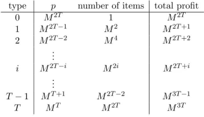
Proof. LetM be a constant larger than 1 (e.g.,M = 10), and consider the following independence system (E,F) (see Table 2).
• The setE consists ofT + 1 types of items, say type 0, type 1, . . . , typeT.
• For eachi= 0,1, . . . , T, type ihasM2i items with profit M2T−i.
Table 2: An independence system with small robustness.
type p number of items total profit
0 M2T 1 M2T
1 M2T−1 M2 M2T+1
2 M2T−2 M4 M2T+2
...
i M2T−i M2i M2T+i ...
T−1 MT+1 M2T−2 M3T−1
T MT M2T M3T
• F is the collection of all the subsets ofE consisting of at most one type of items.
It is not difficult to see thatρ(F) =µ(F) =M2T for this independence system. We show that the robustness of an arbitrary randomized strategy is O(1/T).
For i= 0,1, . . . , T, let Xi be the feasible set consisting of all items of type i. By the definition of F, {X0, X1, . . . , XT} is the set of all maximal feasible sets, and hence it suffices to consider a randomized strategy choosingX0, X1, . . . , XT.
For i, j ∈ {0,1, . . . , T}, we have that p(Xj(M2i)) = M2T+i−|i−j|. Consider a randomized strategy choosing Xj with probabilityλj. Since p(OPTM2i) =M2T+i, it follows that
∑T j=0
λjp(Xj(M2i)) =
∑T
j=0
λjM−|i−j|
·p(OPTM2i) (i= 0,1, . . . , T),
which implies that its robustness is at most mini{∑T
j=0λjM−|i−j| }
. Since
∑T i=0
∑T
j=0
λjM−|i−j|
=
∑T j=0
λj
( T
∑
i=0
M−|i−j| )
≤
∑T j=0
λj (
1 + 2
∑∞ i′=1
M−i′ )
≤1 + 2
M −1 = O(1), the robustness is at most mini
{∑T
j=0λjM−|i−j| }
= O(1/T), which completes the proof.
Theorem 11 shows that the robustness Ω(1/logρ(F)) given in Theorem 10 is tight when we consider general independence systems.
5 Concluding Remarks
In this paper, we have addressed randomized strategies for the robust independence systems de- fined by the knapsack problem. We exhibited upper bounds on robustness in terms of the ex-
changeability µ(F) and a newly introduced parameter ρ(F), which represent the intractability of the independence system (E,F). We then designed randomized strategies with better robustness than deterministic strategies, and extended those results to general independence systems.
A major task for future research would be filling the gap between the upper and lower bounds on robustness. Extending Theorem 6, a lower bound in terms of the exchangeabilityµ(F), to general independence systems, and providing upper or lower bounds in terms of the rank quotientr(F) are also of interest.
References
[1] A. Caprara, H. Kellerer, U. Pferschy and D. Pisinger: Approximation algorithms for knapsack problems with cardinality constraints, European Journal of Operational Research, 123 (2000), 333–345.
[2] R. Fujita, Y. Kobayashi and K. Makino: Robust matchings and matroid intersections, SIAM Journal on Discrete Mathematics, 27 (2013), 1234–1256.
[3] R. Hassin and S. Rubinstein: Robust matchings, SIAM Journal on Discrete Mathematics, 15 (2002), 530–537.
[4] T.A. Jenkyns: The efficiency of the greedy algorithm, in Proceedings of the 7th Southeastern Conference on Combinatorics, Graph Theory, and Computing, Unitas Mathematica, 1976, 341–
350.
[5] N. Kakimura and K. Makino: Robust independence systems,SIAM Journal on Discrete Math- ematics, 27 (2013), 1257–1273.
[6] N. Kakimura, K. Makino and K. Seimi: Computing knapsack solutions with cardinality robust- ness, Japan Journal of Industrial and Applied Mathematics, 29 (2012), 469–483.
[7] B. Korte and D. Hausmann: An analysis of the greedy heuristic for independence systems, Annals of Discrete Mathematics, 2 (1978), 65–74.
[8] J. Matuschke, M. Skutella and J.A. Soto: Robust randomized matchings, in P. Indyk, ed., Proceedings of the 26th Annual ACM-SIAM Symposium on Discrete Algorithms, 2015, 1904–
1915.
[9] J. Mestre: Greedy in approximation algorithms, in Y. Azar and T. Erlebach, eds.,Proceedings of the 14th Annual European Symposium on Algorithms, LNCS 4168, Springer-Verlag, 2006, 528–539.