R ESEARCH I NSTITUTEFOR M ATHEMATICAL S CIENCESKYOTOUNIVERSITY,Kyoto,Japan BySakieSUZUKINovember2011 OnthecoloredJonespolynomialsofribbonlinks,boundarylinksandBrunnianlinks RIMS-1733

RIMS-1733

On the colored Jones polynomials

of ribbon links, boundary links and Brunnian links

By

Sakie SUZUKI

November 2011

R _ESEARCH I NSTITUTE FOR M ATHEMATICAL S _CIENCES

On the colored Jones polynomials of ribbon links, boundary links and Brunnian links

Sakie Suzuki

November 27, 2011

Abstract

Habiro gave principal ideals of Z[q, q⁻¹] in which certain linear combinations of the colored Jones polynomials of algebraically-split links take values. The author proved that the same linear combinations for ribbon links, boundary links and Brunnian links are contained in smaller ideals ofZ[q, q⁻¹] generated by several elements. In this paper, we prove that these ideals also are principal, each generated by a product of cyclotomic polynomials.

1 Introduction

After the discovery of the Jones polynomial, Reshetikhin and Turaev [7] defined an invariant of framed links whose components are colored by finite dimensional represen- tations of a ribbon Hopf algebra. Thecolored Jones polynomial can be defined as the Reshetikhin-Turaev invariant of links whose components are colored by finite dimen- sional representations of the quantized enveloping algebraUh(sl2).

We are interested in the relationship between algebraic properties of the colored Jones polynomial andtopological properties of links.

In this paper, we consider the following three types of links.

A link is called aribbon link if it bounds the image of an immersion from a disjoint union of disks intoS³with only ribbon singularities.

Ann-component linkL=L₁∪· · ·∪L_nis called aboundary linkif it bounds a disjoint union ofnSeifert surfacesF1, . . . , Fn inS³ such thatLi boundsFi fori= 1, . . . , n.

A linkLis called aBrunnian link if every proper sublink ofLis trivial.

In [4], Habiro used certain linear combinations J_{L; ˜P}′

l1,...,P˜_ln^′ , l1, . . . , ln ≥ 0, of the colored Jones polynomials of a link L to construct the unified Witten-Reshetikhin- Turaev invariants for integral homology spheres. He proved that J_{L; ˜P}′

l1,...,P˜^′

ln

for an algebraically-split, 0-framed linkL is contained in a certain principal ideal ofZ[q, q⁻¹] (Theorem 2.1). This result was improved by the present author [8, 9, 10, 11] in the

∗Research Institute for Mathematical Sciences, Kyoto University, Kyoto, 606-8502, Japan. E-mail address:[email protected]

special case of ribbon links, boundary links (Theorem 2.2) and Brunnian links (Theorem 2.4) by using idealsIl₁, . . . , Il_n ofZ[q, q⁻¹], where Theorem 2.2 for boundary links had been conjectured by Habiro [4]. Here, in [8], we gave an alternative proof of the fact that the Jones polynomial of ann-component ribbon link is divisible by the Jones polynomial of the n-component trivial link, which was proved first by Eisermann [1]. The results in [4, 8, 9, 10, 11] are proved by using theuniversalsl₂ invariant of bottom tangles(cf.

[3, 4]), which has the universality property for the colored Jones polynomial of links.

In this paper, we prove that the ideal I_l, l ≥0, is a principal ideal generated by a product of cyclotomic polynomials (Theorem 3.1), and rewrite Theorems 2.1, 2.2 and 2.4 by using these generators (Proposition 3.3).

2 Results for the colored Jones polynomial

In this section, we recall results in [4, 9, 10, 11] for the colored Jones polynomial. For the definition of the quantized enveloping algebra U_h(sl₂), see, e.g., [6, 4, 9]. We set q= exph.

For m≥1, let Vmdenote the m-dimensional irreducible representation ofUh(sl2).

LetRdenote the representation ring ofUh(sl2) overQ(q¹²), i.e.,Ris theQ(q¹²)-algebra R= Span

Q(q¹2){V_m |m≥1}

with the multiplication induced by the tensor product. It is well known that R = Q(q¹²)[V2].

Habiro [4] studied the following elements inR P˜_l^′= q^12l

{l}q!

l−1

∏

i=0

(V2−qⁱ⁺¹² −q⁻ⁱ⁻¹²),

forl≥0,which are used in an important technical step in his construction of the unified Witten-Reshetikhin-Turaev invariants for integral homology spheres.

For the definition of the colored Jones polynomialJL;X₁,...,X_n ofLwithith compo- nentLi colored byXi∈ R, see, e.g., [5, 4, 9].

Set

{i}q =qⁱ−1, {i}q,n={i}q{i−1}q· · · {i−n+ 1}q, {n}q! ={n}q,n, fori∈Z, n≥0.

Habiro [4] proved the following.

Theorem 2.1 (Habiro [4]). Let L be an n-component, algebraically-split link with 0- framing. We have

J_{L; ˜P}′

l1,...,P˜_ln^′ ∈ {2lmax+ 1}q,l_max+1

{1}q

Z[q, q⁻¹], (1)

forl1, . . . , ln ≥0, wherelmax= max(l1. . . , ln).

Set

fl,k={l−k}q!{k}q!,

for 0≤k≤l. Forl≥0, letI_l be the ideal ofZ[q, q⁻¹] generated byf_l,0, . . . , f_l,l. In [9, 10], we proved the following.

Theorem 2.2 ([9, 10]). Let L be an n-component ribbon or boundary link with 0- framing. Forl₁, . . . , l_n≥0, we have

J_{L; ˜P}′

l1,...,P˜_ln^′ ∈ {2lmax+ 1}q,l_max+1

{1}q

∏

1≤i≤n,i̸=i_M

Il_i, (2)

wherelmax= max(l1, . . . , ln)andiM is an integer such thatli_M =lmax.

Remark 2.3. Theorem 2.2 for boundary links had been conjectured by Habiro [4].

In [11], we prove the following.

Theorem 2.4([11]). LetL be an n-component Brunnian link withn≥3. We have J_{L; ˜P}′

l1,...,P˜^′

ln ∈ {2lmax+ 1}q,lmax+1

{1}q{lmin}q!

∏

1≤i≤n,i̸=iM,im

Il_i, (3)

for l1, . . . , ln ≥ 0, where lmax = max(l1, . . . , ln), lmin = min(l1, . . . , ln) and iM, im, iM ̸=im, are integers such thatli_M =lmax,li_m =lmin, respectively.

Let us compare Theorems 2.1, 2.2 and 2.4. Forl1, . . . , ln ≥0, letZa^(l1,...,ln),Z_r,b^(l1,...,ln) andZ_Br^(l1,...,ln)denote the ideals ofZ[q, q⁻¹] at the right hand sides of (1), (2) and (3), respectively, i.e., we set

Z_a^(l1,...,ln)= {2lmax+ 1}q,l_max+1

{1}q Z[q, q⁻¹], Z_r,b^(l1,...,ln)= {2lmax+ 1}q,lmax+1

{1}q

∏

1≤i≤n,i̸=iM

Il_i,

Z_Br^(l1,...,ln)= {2l_max+ 1}q,lmax+1

{1}q{lmin}q!

∏

1≤i≤n,i̸=iM,im

I_li.

Forl1, . . . , ln≥0, we have

Z_r,b^(l1,...,ln)⊂Z_a^(l1,...,ln), Z_r,b^(l1,...,ln)⊂Z_Br^(l1,...,ln), since we have

Z_r,b^(l1,...,ln)=( ∏

1≤i≤n,i̸=i_M

I_li)

·Z_a^(l1,...,ln),

=(

{l_min}q!I_lmin)

·Z_Br^(l1,...,ln).

On the other hand, there are no inclusion which satisfies for alll1, . . . , ln≥0 between Za^(l1,...,ln) and Z_Br^(l1,...,ln) . For example, we have Za^(2,2,2,2) ̸⊂Z_Br^(2,2,2,2) and Z_Br^(2,2,2,2) ̸⊂

Za^(2,2,2,2) since

Z_a^(2,2,2,2)= {5}q,3

{1}q Z[q, q⁻¹]

= (q−1)²(q+ 1)(q²+q+ 1)(q²+ 1)(q⁴+q³+q²+q¹+ 1)Z[q, q⁻¹], Z_Br^(2,2,2,2)= {5}q,3

{1}q{2}q!{1}⁴qZ[q, q⁻¹]

= (q−1)⁴(q²+q+ 1)(q²+ 1)(q⁴+q³+q²+q¹+ 1)Z[q, q⁻¹].

Since a Brunnian link withn≥3 components is algebraically-split with 0-framing, we have the following refinement of Theorem 2.4.

Theorem 2.5. Let Lbe an n-component Brunnian link withn≥3. We have J_{L; ˜P}′

l1,...,P˜_ln^′ ∈Z_a^(l1,...,ln)∩Z_Br^(l1,...,ln), forl₁, . . . , l_n ≥0.

3 Main result for the ideal I

In this section, we state the main result of this paper.

Forl≥0, recall the generatorsf_l,0, . . . , f_l,l of the ideal I_l. Set gl=GCD(fl,0, . . . , fl,l).

It is clear that Il ⊂ glZ[q, q⁻¹]. The opposite inclusion follows if and only if Il is principal. Since Z[q, q⁻¹] is not a principal ideal domain, it had been a problem ifIl

is principal or not. The main result in this paper (Theorem 3.1) is thatIl is principal, where we determineglexplicitly. The proof is in Section 4.

Form≥1, let Φm=∏

d|m(q^d−1)^µ(md)∈Z[q] denote themth cyclotomic polynomial, where∏

d|mdenotes the product over all positive divisors dofm, and µis the M¨obius function. Forr∈Q, we denote by⌊r⌋the largest integer smaller than or equal tor.

Theorem 3.1. Forl≥0, the idealI_l is the principal ideal generated byg_l. Moreover, we have

gl= ∏

m≥1

Φ^tm^l,m, (4)

where

tl,m=

{⌊^l+1_m ⌋ −1 for1≤m≤l,

0 forl < m.

Here is a table oftl,m for 1≤m≤4, 0≤l≤16.

m\l 0 1 2 3 4 5 6 7 8 9 10 11 12 13 14 15 16

1 0 1 2 3 4 5 6 7 8 9 10 11 12 13 14 15 16

2 0 0 0 1 1 2 2 3 3 4 4 5 5 6 6 7 7

3 0 0 0 0 0 1 1 1 2 2 2 3 3 3 4 4 4

4 0 0 0 0 0 0 0 1 1 1 1 2 2 2 2 3 3

Remark 3.2. In [11], Theorem 3.1 is used in the proof of Theorem 2.4.

Theorem 3.1 implies that the idealsZ_r,b^(l1,...,ln)andZ_Br^(l1,...,ln)are principal. Moreover, we can write a generator of each principal idealZa^(l1,...,ln),Z_r,b^(l1,...,ln)andZ_Br^(l1,...,ln)as a product of cyclotomic polynomials as follows.

Proposition 3.3. Forl1, . . . , ln ≥0, the idealsZa^(l1,...,ln), Z_r,b^(l1,...,ln) andZ_Br^(l1,...,ln) are principal. Moreover, we have

Z_a^(l1,...,ln)= ∏

m≥1

Φ^⌊

2lmax +1

m ⌋−⌊^lmax−1m ⌋−⌊m¹⌋

m Z[q, q⁻¹],

Z_r,b^(l1,...,ln)= ∏

1≤m≤2l_max+1

Φ^⌊

2lmax +1

m ⌋−⌊^lmax−m ¹⌋−⌊m¹⌋+∑

1≤i≤n,i̸=iMt_li,m

m Z[q, q⁻¹],

Z_Br^(l1,...,ln)= ∏

1≤m≤2lmax+1

Φ^⌊

2lmax +1

m ⌋−⌊^lmax−1m ⌋−⌊m¹⌋−⌊^lminm ⌋+∑

1≤i≤n,i̸=iM ,imt_li,m

m Z[q, q⁻¹].

Proof. The assertion forZa^(l1,...,ln)follows from {l}q,i= ∏

m≥1

Φ^⌊m^{ml⌋−⌊l−im⌋}, (5)

for 0≤i≤l. The assertion for Z_r,b^(l1,...,ln) and Z_Br^(l1,...,ln) follows from (5) and Theorem 3.1.

Corollary 3.4. Forl₁, . . . , l_n≥0, we have Z_a^(l1,...,ln)∩Z_Br^(l1,...,ln)= ∏

m≥1

Φ^⌊

2lmax +1

m ⌋−⌊^lmax−1m ⌋−⌊m¹⌋+max(0,∑

1≤i≤n,i̸=iM ,imt_li,m−⌊^lminm ⌋)

m Z[q, q⁻¹].

Example 3.5. Let L be an n-component algebraically-split link with 0-framing. By Theorem 2.1 and Proposition 3.3, we have

J_{L; ˜P}′

1,...,P˜₁^′ ∈Φ1Φ2Φ3Z[q, q⁻¹], J_{L; ˜P′}

2,...,P˜₂^′ ∈Φ²₁Φ₂Φ₃Φ₄Φ₅Z[q, q⁻¹], J_{L; ˜P}′

3,...,P˜₃^′ ∈Φ³₁Φ²₂Φ3Φ4Φ5Φ6Φ7Z[q, q⁻¹].

...

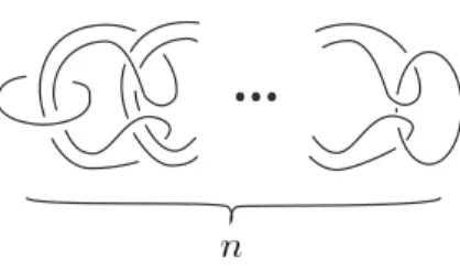
Figure 1: Milnor’s linkMn

Let Lbe an n-component Brunnian link withn≥3. By Theorem 2.5 and Corollary 3.4, we have

J_{L; ˜P}′

1,...,P˜₁^′ ∈Φ₁ⁿ⁻²Φ2Φ3Z[q, q⁻¹], J_{L; ˜P}′

2,...,P˜₂^′ ∈Φ²⁽ⁿ₁ ⁻²⁾Φ₂Φ₃Φ₄Φ₅Z[q, q⁻¹], J_{L; ˜P}′

3,...,P˜₃^′ ∈Φ³⁽ⁿ₁ ⁻²⁾Φ₂ⁿ⁻¹Φ3Φ4Φ5Φ6Φ7Z[q, q⁻¹].

Let Lbe an n-component ribbon or boundary link with0-framing. By Theorem 2.2 and Proposition 3.3, we have

J_{L; ˜P′}

1,...,P˜₁^′ ∈Φ₁ⁿΦ₂Φ₃Z[q, q⁻¹], J_{L; ˜P}′

2,...,P˜₂^′ ∈Φ²ⁿ₁ Φ2Φ3Φ4Φ5Z[q, q⁻¹], J_{L; ˜P}′

3,...,P˜₃^′ ∈Φ³ⁿ₁ Φⁿ⁺¹₂ Φ3Φ4Φ5Φ6Φ7Z[q, q⁻¹].

Example 3.6. Forn≥3, let M_n be Milnor’sn-component Brunnian link depicted in Figure 1. Note thatM3 is the Borromean rings. We have

J_M

n; ˜P₁^′,...,P˜₁^′ = (−1)ⁿq⁻²ⁿ⁺⁴Φⁿ₁⁻²Φ₂ⁿ⁻²Φ3Φⁿ₄⁻³,

which we will prove in a forthcoming paper [12]. This implies that Theorem 2.4 is best possible for the divisibility by Φ1 and Φ3 of J_{L; ˜P}′

1,...,P˜₁^′ with L Brunnian. By Theorem 2.2, this also implies that eachM_n is not ribbon or boundary.

4 Proof of Theorem 3.1

We prove Theorem 3.1.

For a1, . . . , am ∈ Z[q, q⁻¹], let (a1, . . . , am) denote the ideal in Z[q, q⁻¹] generated bya₁, . . . , a_m∈Z[q, q⁻¹].

Forl≥0, recall thatI_l= (f_l,0, f_l,1, . . . , f_l,l) withf_l,i={l−i}q!{i}q! for 0≤i≤l.

For 0≤k≤l, we have

(fl,0, fl,1, . . . , fl,k) ={l−k}q!(hl,k,0, hl,k,1, . . . , hl,k,k) with

hl,k,i=fl,i/{l−k}q!

={l−i}q,k−i{i}q!,

for 1≤i≤k.

Set

I_l,k= (h_l,k,0, h_l,k,1, . . . , h_l,k,k), gl,k=GCD(hl,k,0, hl,k,1, . . . , hl,k,k).

Note thatIl,l=Il andgl,l=gl.

In what follows, for a ∈ Z[q, q⁻¹]\ {0} and m ≥ 1, let dm(a) denote the largest integerisuch thata∈Φⁱ_mZ[q, q⁻¹]. For 0≤k≤l, we can write

gl,k= ∏

m≥1

Φ^dm^m(gl,k), since eachhl,k,iis a product of cyclotomic polynomials.

Lemma 4.1. For0≤k≤l, we have dm(gl,k) =

{⌊^l+1_m ⌋ −1− ⌊^l_m^−k⌋ for1≤m≤k,

0 fork < m.

Proof. We have

dm(gl,k) = min{dm

(hl,k,i

)|0≤i≤k}

= min{dm

({l−i}q,k−i{i}q!)

|0≤i≤k}

= min{⌊l−i

m ⌋ − ⌊l−k m ⌋+⌊i

m⌋|0≤i≤k}

= min{⌊l−i m ⌋+⌊ i

m⌋|0≤i≤k} − ⌊l−k m ⌋. Ifk < m, then we havedm(gl,k) = 0 sincedm

(hl,k,k) =dm

({k}q!) = 0.

Let 1≤m≤k. Since we have

⌊l−(i+am)

m ⌋+⌊i+am

m ⌋=⌊l−i m ⌋+⌊i

m⌋, for 0≤i≤kanda∈Z, we have

min{⌊l−i m ⌋+⌊i

m⌋|0≤i≤k}= min{⌊l−i m ⌋+⌊i

m⌋|0≤i≤m−1}.

Here, for 0≤i≤m−1, we have⌊_mⁱ⌋= 0 and⌊^l−_mⁱ⌋takes the minimum withi=m−1.

Thus we have

min{⌊l−i m ⌋+⌊i

m⌋|0≤i≤m−1}=⌊l−(m−1)

m ⌋

=⌊l+ 1 m ⌋ −1.

This implies

dm(gl,k) =⌊l+ 1

m ⌋ −1− ⌊l−k m ⌋. Hence we have the assertion.

Note that we have the latter part (4) of Theorem 3.1 as follows.

Corollary 4.2. Forl≥0, we have

gl=gl,l = ∏

m≥1

Φ^tm^l,m.

From now, we prove the following generalization of Theorem 3.1.

Proposition 4.3. For0≤k≤l, the idealIl,k is the principal ideal generated bygl,k. For 1≤k≤l, set

˜

g_l,k=g_l,k/g_l,k−1. We have

˜

g_l,k= ∏

1≤m≤k

Φ^⌊

l+1

m ⌋−1−⌊^l−k_m ⌋−(

⌊^l+1_m ⌋−1−⌊^l−k+1_m ⌋)

m

= ∏

1≤m≤k

Φ^⌊m^{l−k+1m ⌋−⌊l−km ⌋}

= ∏

m|l−k+1 1≤m≤k

Φ_m.

We use the following technical lemma.

Lemma 4.4. For1≤k≤l, we have

({l−k+ 1}q,{k}q{k−1}q!

g_l,k−1 ) = (˜gl,k).

(Note thatgl,k−1=GCD({l}q,k−1,{l−1}q,k−2{1}q, . . . ,{k−1}q!) divides{k−1}q!.) Proof of Proposition 4.3 by assuming Lemma 4.4 . We use induction on k. For k= 0, clearly we have

I_l,0= (g_l,0) = ({l}q!).

Fork≥1, we have

I_l,k= (h_l,k,0, h_l,k,1, . . . , h_l,k,k)

= ({l}q,k,{l−1}q,k−1{1}q, . . . ,{l−k+ 1}q{k−1}q!,{k}q!)

=(

{l−k+ 1}q({l}q,k−1,{l−1}q,k−2{1}q, . . . ,{k−1}q!),{k}q!)

= ({l−k+ 1}qg_l,k−1,{k}q!)

=gl,k−1({l−k+ 1}q,{k}q{k−1}q! g_l,k−1 )

= (gl,k−1g˜l,k)

= (g_l,k),

where the second equality is given by

h_l,k,0={l−k+ 1}q· {l−i}q,k−i−1{i}q,

for 0≤i≤k−1, and the third equality is given by the assumption of the induction.

Hence we have the assertion.

In what follows, we prove Lemma 4.4. We use the following two lemmas, which are well-known.

Lemma 4.5 (cf. Habiro [2, Lemma 4.1]). For a, b ≥ 0, the following conditions are equivalent.

(i) (Φa,Φb) =Z[q, q⁻¹]

(ii) ^a_b ̸=pⁱ for any prime number p≥0 andi∈Z

Lemma 4.6. Let a₁, . . . , a_m, b₁, . . . , b_n ∈Z[q, q⁻¹]such that (a_i, b_j) =Z[q, q⁻¹]for all 1≤i≤m,1≤j≤n. We have

(a1a2· · ·am, b1b2· · ·bn) =Z[q, q⁻¹].

Proof of Lemma 4.4. It is enough to prove the following two equalities.

GCD({l−k+ 1}q,{k}q{k−1}q! gl,k−1

) = ˜gl,k, (6)

({l−k+ 1}q/˜g_l,k,{k}q

{k−1}q! gl,k−1

/˜g_l,k) =Z[q, q⁻¹], (7) for 1≤k≤l.

First, we prove (6). Recall that

˜

gl,k= ∏

m|l−k+1 1≤m≤k

Φm. (8)

Since{l−k+ 1}q=∏

m|l−k+1Φm anddm({k}q{k−1}q!

g_l,k−1 ) = 0 form > k, it is enough to check

d_m({k}q

{k−1}q! gl,k−1

)≥1, form|l−k+ 1, 1≤m≤k. Indeed, we have

d_m({k}q) = {

1 form|k,

0 form̸ |k, (9)

dm({k−1}q! g_l,k−1 ) =

{

0 form|k,

1 form̸ |k. (10)

Here, (9) is clear and (10) follows from d_m({k−1}q!

gl,k−1

) =⌊k−1

m ⌋ −t_l,k−1,m

=⌊k−1

m ⌋ − ⌊l+ 1

m ⌋+ 1 +⌊l−k+ 1

m ⌋

=⌊pm+r−1

m ⌋ − ⌊(p+p^′)m+r

m ⌋+ 1 +⌊p^′m m ⌋

=⌊r−1 m ⌋+ 1

= {

0 forr= 0,

1 for 1≤r≤m−1,

where, we writek=mp+r andl−k+ 1 =mp^′ withp, p^′≥1 and 0≤r≤m−1.

We prove (7). By Lemmas 4.5 and 4.6, it is enough to prove that there are no pair of integersm, n≥1 such that

• _mⁿ =pⁱ for a primepandi∈Z,

• d_m({l−k+ 1}q/˜g_l,k)≥1, and

• d_n({k}q{k−1}q!

g_l,k−1 /˜g_l,k)≥1.

Note that

{l−k+ 1}q/˜g_l,k= ∏

m|l−k+1 m>k

Φ_m.

Letm|l−k+ 1, m > k. Recall that forn > k, we haved_n({k}q{k−1}q!

g_l,k−1 ) = 0. Assume that 1 ≤n ≤ k and n|m, which implies n|l−k+ 1. The conditions 1 ≤ n ≤k and n|l−k+ 1 implydn(˜gl,k−1) = 1 by (8). By (9) and (10), we havedn({k}q{k−1}q!

g_l,k−1 ) = 1.

Thus we havedn({k}q{k−1}q!

g_l,k−1 /g˜l,k) = 0, which completes the proof.

Acknowledgments. This work was partially supported by JSPS Research Fellowships for Young Scientists. The author is deeply grateful to Professor Kazuo Habiro and Professor Tomotada Ohtsuki for helpful advice and encouragement.

References

[1] M. Eisermann, The Jones polynomial of ribbon links. Geom. Topol. 13 (2009), no. 2, 623–660.

[2] K. Habiro, Cyclotomic completions of polynomial rings. Publ. Res. Inst. Math. Sci.

40(2004), no. 4, 1127–1146.

[3] K. Habiro, Bottom tangles and universal invariants. Alg. Geom. Topol. 6(2006), 1113–1214.

[4] K. Habiro, A unified Witten-Reshetikhin-Turaev invariants for integral homology spheres. Invent. Math.171(2008), no. 1, 1–81.

[5] V. F. R. Jones, Hecke algebra representations of braid groups and link polynomials.

Ann. Math. (2)126(1987), 335–388.

[6] C. Kassel, Quantum groups. Graduate Texts in Mathematics,155, Springer-Verlag, New York, 1995.

[7] N. Y. Reshetikhin, V. G. Turaev, Ribbon graphs and their invariants derived from quantum groups. Comm. Math. Phys.127(1990), no. 1, 1–26.

[8] S. Suzuki, Master’s thesis. Kyoto university, 2009.

[9] S. Suzuki, On the universalsl2 invariant of ribbon bottom tangles. Algebr. Geom.

Topol.10(2010), no. 2, 1027–1061.

[10] S. Suzuki, On the universal sl2 invariant of boundary bottom tangles.

arXiv:1103.2204.

[11] S. Suzuki, On the universalsl₂ invariant of Brunnian bottom tangles. In prepara- tion.

[12] S. Suzuki, In preparation.