Licensing and R&D Investment of Duopolistic
Firms with Partially Complementary
Technologies
journal or
publication title
Discussion paper series
number
25
page range
1-53
year
2005-03-14
DISCUSSION PAPER SERIES
Discussion paper No.25
Licensing and R&D Investment of Duopolistic Firms
with Partially Complementary Technologies
Tetsuya Shinkai Kwansei Gakuin University
Satoru Tanaka
Kobe City University of Foreign Studies and
Makoto Okamura ,iroshima University
March 2005
SCHOOL OF ECONOMICS
KWANSEI GAKUIN UNIVERSITY
1-155 Uegahara Ichiban-cho Nishinomiya 662-8501, Japan
Licensing and R&D Investment of Duopolistic Firms with Partially
Complementary Technologies
*Tetsuya Shinkai, Kwansei Gakuin University, Satoru Tanaka, Kobe City University of Foreign Studies
and
Makoto Okamura, Hiroshima University
March 14, 2005
Abstract
We consider research and development (R&D) investment competition between duopolistic firms that independently invest in two complementary technologies to produce their products. By “partially
complementary technologies”, we mean that each firm can produce the goods without both technologies but
they incur more redundant costs than with both technologies. We derive the investment competition equilibria in R&D of the two technologies with and without a licensing system. By comparing R&D investment levels in the two equilibria, we show that the licensing system discourages R&D investment in most cases; however, it encourages R&D investment in some cases when the duopolistic firms can produce the goods using both technologies. We also show that (cross-) licensing increases the expected social surplus at the symmetric equilibrium.
JEL Classification Numbers: D45, L13, O32
Key Words: partially complementary technologies, licensing system, duopoly, R&D investment
Corresponding To: Tetsuya shinkai, ph D, 1-155, Uegahara-ichibancho, Nishinomiya, Hyogo 662-8501, JAPAN
E-mail: [email protected], FAX 81-798-51-0944
* We are very grateful to Kaori Hatanaka, Hiroshi Izawa, Toshihiro Matsumura, Keizo Mizuno, Sadao Nagaoka, Hiroyuki Odagiri, Kuninobu Takeda, and the participants in the Contract Theory Workshop (CTW) held at Kyoto Institute’s Economic Research, and the Microeconomics Workshop held in the Center for International Research on the Japanese Economy at the University of Tokyo, for their valuable comments and discussion on earlier versions of this work. This research was supported by a grant-in-aid from the Zengin Foundation for Studies on Economics and Finance and by a Grant-in-Aid for Scientific Research number 14530066 from the Ministry of
1. Introduction
One significant feature of recent technological innovation is that a firm often employs multiple distinct technologies to produce a commodity. Especially in information technology (IT) industries, one product is composed of numerous separable patentable elements. For example, the production of a mobile phone with a digital camera involves about 19,000 (Japanese) patents and/or utility models.1 In this environment, which has been called “cumulative-systems technologies” (Merges and Nelson (1994)) or “complex technologies” (Cohen, Nelson and Walsh (2000)), many economic agents hold and share the separable patentable elements. The method of coordination among these patent holders affects the interests of each inventor and also affects their R&D incentives. Over the last decade of the previous century, a number of studies have discussed the effects on R&D activities, licensing and the patent systems of the mode of coordination of inventions.
Considering complex technologies, we can identify in principle two types of relationships between inventions. The first type is cumulative or one-way complementary. As Scotchmer (1991) pointed out, many inventors engage in R&D activities based on the outcome of preceding inventions. Here, while an applied technology invention that is based on basic technologies is not possible without the existence of these basic technologies, invention of the basic technologies in themselves is possible without the outcome of the applied technologies. With respect to this relationship, Green and Scotchmer (1995), and Chang (1995) showed that externalities, due to the lack of coordination among the creators of plural distinct inventions, discourage the development of these technologies. In the second type of relationship among inventions, various mutually interdependent inventions are required, without which production of the goods is very difficult. Thus, this relationship among inventions is called two-way complementary.
1
In fact, as we have seen typically in the IT industries, technological innovations occur on the basis of plural distinct inventions developed in different systems of technologies. Distinct technologies are complementary to each other as parts of the product produced. An externality problem occurs due to a lack of coordination among the discoverers of plural complementary technologies. Heller and Eisenberg (1998) stated that the existence of such externality results in “the tragedy of anti-commons”. When the intellectual property rights of plural distinct technologies are assigned to different agents (firms), the externality generates excessive exercises of exclusive rights and leads to under-utilization of these technologies, and this under-utilization discourages R&D activities of agents (firms).
When all complementary technologies are necessary to produce a product, licensing has strategic importance. If two firms own each of two distinct inventions with complete complementarity, then the two firms cannot produce a product at all without a cross-licensing contract. The form of this coordination affects R&D activities of the firms. Grindley and Teece (1997) and Hall and Ziedonis (2001) conducted empirical investigations of the appliance and integrated circuit (IC) industries. Their results show the conditions of the firms’ (cross-) licensing of technologies have a significant effect on the incentives for R&D activities in these industries where complementary inventions are indispensable for production. While there are many empirical studies on this subject, few theoretical studies have examined how the conditions of firms’ (cross-) licensing of technologies affect firms’ incentives for R&D activities. Fershtman and Kamien (1992) and Okamura, Shinkai and Tanaka (2002) offer two of the few studies of two firms engaging in R&D activities for two distinct technological inventions with complete complementarity. They both established that the existence of a cross-licensing system reduces the firms’ R&D activities in such a context.
Complementary technological inventions are not always indispensable for production, in which case firms may produce a new product without using any one of two complementary inventions. For example, in IC technologies, a great number of distinct technological
inventions with complementarity exist such as software technologies, liquid crystal display (LCD) technologies and so on, all of which are indispensable for producing a mobile phone. Some firms, however, can develop and produce a new and superior mobile phone by using the outcomes of the successful invention with regard to software technologies and LCD technologies. In this environment, the margin created by the cost reduction (e.g. of the mobile phone) depends on the degree of complementarity of the underlying technologies. When the degree of complementarity is large (small), we expect that the cost reduction created by invention of only one element of the underlying technologies is small (large). Such an environment opens the possibility of unilateral licensing for coordinating technological inventions. When firms invest in R&D in two distinct technologies with complete complementarity, both technologies are indispensable for producing products, and the realized pattern of licensing becomes cross-licensing. On the contrary, consider the invention of one element of the underlying technologies that is dispensable for production but also contributes to cost reduction. This invention may be unilaterally licensed. Therefore, we employ a static framework to examine how the degree of complementarity between underlying technologies and the difference between cross-licensing and unilateral licensing changes firms’ incentives for R&D activities in a Cournot duopoly. We concentrate on the case where each duopolistic firm can invest in R&D for two distinct technological inventions with partial complementarity with each other.
In Section 2, we describe our model. In Section 3, we analyze the problem of R&D in a Cournot duopoly with partially complementary technological innovations without licensing as a benchmark. In Section 4, we examine the conditions under which (cross-) licensing occurs. The appendix presents the conditions under which (cross-) licensing may occur at every state of nature. After extending our analysis to the case of (cross-) licensing in Section 5, we analyze theoretically how the difference between cross-licensing and unilateral licensing affects firms’ incentives for R&D activities in a Cournot duopoly in Sections 5 and 6. In
Section 7, we use a numerical example to discuss briefly how the difference between cross-licensing and unilateral licensing affects welfare at the equilibria. In the final section, we present our concluding remarks.
2. The model
We consider a duopolistic market in which two firms with identical production technology, firms x and y, produce a homogeneous product. At the first stage, each firm simultaneously invests in R&D for the two distinct but partially complementary technologies,
A and B. By “partially complementary technologies,” we mean that each firm can produce the
goods without both two technologies but it incurs additional costs than with both technologies. Denote by xA, xB(≥ 0) and yA,yB(≥0) the investment levels for the technologies A, B of firm x and those for the technologies A, B of firm y. If each firm succeeds in the development of at least one of these technologies, it can reduce marginal cost through a process innovation. Assume that each firm has a constant return to scale production technology as follows:
i i
i i
i q cq c q
C ( )= =( +0)⋅ , if it succeeds in the development of both technologies A and B,
=(c+k)⋅qi, if it succeeds in the development of technologies A or B, where 0≤ k ≤1,
i
q
c+ ⋅
=( 1)
, if it fails to develop both technologies A and B
y x
i = , , (1)
where c is an intrinsic marginal cost and we set c = 0 without loss of generality.
This cost function implies that marginal cost decreases by 1, 1−k and 0 if firmi(=x,y)succeeds in the development of both, either and none of the two technologies. We say the two technologies A and B are less partially complementary, even partially
respectively. Especially, the two technologies are the least partially complementary or the
most partially complementary, if k = 0 or k = 1.2
If each firm succeeds in the development of either technology A or B, it can reduce its marginal cost by 1−k. If it succeeds in the development of both technologies, the firm can reduce its marginal cost by 1. Suppose that the firm can develop the two technologies sequentially. This implies that the later developed technology decreases marginal cost by k, which is the value of the development of the second technology. Hence, if 1 2< k≤1, the second technology reduces marginal cost more than does the first. In that case, increasing returns to R&D activity occurs. If k =12, the values of both technologies are equivalent. If
2 1
0≤ k< , the R&D technologies exhibit decreasing returns. At the end of the first stage, “nature” chooses whether each firm succeeds in developing the technologies or not. Suppose that each firm succeeds in the development of the technology j with probability and assume that pj(⋅) are identically and independently distributed. Therefore, we have
B A j e z p e y p e x p y z j y x j x j j ( ) 1 ( ) 1 , , 1 )
( = − − = = − − = = − − = . These probability functions are well defined since we have
∞ → ′ < ⋅ ″ > ⋅ ′() 0,p () 0,p (0) p andp(0)=0,p(∞)=1.3
The inverse market demand function for the product is given by
Q a
p= − , (2)
2 That is, we distinguish “the most partially complementary technologies” from “completely complementary technologies”; that is, the latter implies that no firm can produce the goods at all without the use of both
technologies. In this paper, “completely complementary technologies” is expressed by the case where the
marginal cost k is infinitely large; that is k →∞. Okamura, Shinkai and Tanaka (2002) analyzed the case of completely complementary technologies.
3 We assume the effect of the R&D activity on a process innovation as static. That is, the successes or failures of the development do not obey a stochastic process. However, these properties of the success probability function are similar to the dynamic “memoryless” or “Poisson” patent race model associated with Reinganum (1982). In her model of the research technology, it is assumed that a firm’s probability of making a discovery and obtaining a patent at a point of time depends only on this firm’s current R&D investment level and not on its past R&D
where p is the market price and Q is the aggregate output in the market, that isQ=qx+qy. We assume that the market is sufficiently large, i.e.
2 4 39 k
a≥ − . At the beginning of the second stage, each firm knows all successes or failures of the both firms’ developments of the technologies. At the second stage, if a (cross-) licensing system is available, then each firm bargains with its rival and agrees on a (cross-) licensing contract through the Nash bargaining process. The licensing contract describes how both firms divide the total profit. If a (cross-) licensing system is not available, then the game proceeds to the third stage. At the third stage, each firm’s marginal cost is realized and it chooses its output simultaneously, that is, Cournot competition occurs.4 Finally, the profit of each firm is realized and the game is over. The timing of the game is illustrated in Figure 1.
Let us conduct some preliminary work. Denote firm i ’s profit byπi(qi,qj). ) , , ( ) ( ) , (qi qj a qi qj ci qi i j i x y i = − − − ≠ = π , (3)
where }ci =c∈{ k0, ,1 . Since each firm engages in Cournot competition, the equilibrium output of firm i is given by
3 ) 2 ( ) , ( * i j j i i c c a c c q = − + i,j= x,y,i≠ j. (4)
(The first stage ) (The second Stage) (The third stage) Decision on R&D Bargaining for licensing Decision on quantity
investment level and choice of the license fee of outputs
Cournot competition Nature’s choice on success
or failure of the development
4 Note that each firm can produce its product by using its own existing technology, even if it fails to develop both technologies, A and B in our model.
Figure 1. Timing of the game
Substituting (4) into (3) yields firm i ’s Cournot equilibrium profit,
2 * * 3 2 )) , ( ), , ( ( ) , ( ⎟⎟ ⎠ ⎞ ⎜⎜ ⎝ ⎛ − + = ≡ i j i j j j i i i j i i c c a c c q c c q c c π π . (5)
3. R&D investment without (cross-) licensing: A benchmark
In this section, as a benchmark, we analyze the problem of R&D in a Cournot duopoly with partially complementary technological innovation without licensing.5
Denote by {X,Y}, the combination of the states of nature which firms x and y face: Where X,Y∈{AB,A,B,φ} and “AB”, “A”, “B” and “φ” implies that each firm succeeds in development of technologies A and B, A or B and neither A nor B. All possible states of nature are as follows: {AB, AB}, {AB, A}, {AB, B}, {AB, φ}, {A, AB}, {A, A}, {A, B}, {A,φ}, {B,
AB}, {B, A}, {B, B}, {B, φ}, {φ, AB}, {φ, A}, {φ, B} and {φ, φ}.6
For these states of nature, the corresponding realized equilibrium firm x’s profits are ) 1 , 0 ( ), , 0 ( ), , 0 ( ), 0 , 0 ( x x x x π k π k π π , πx(k,0),πx(k,k),πx(k,k),πx(k,1) , πx(k,0),πx(k,k) , ) 1 , ( ), , (k k x k x π π ,πx(1,0),πx(1,k),πx(1,k)and )πx(1,1 .
The expected profit of firm x without (cross-) licensing is given by ) , , , ( A B A B x x≡EΠ x x y y
Π
=(1−e−xA)(1−e−xB)H1+ 2 ) 1 ( −e−xA e−xBH +e−xA(1−e−xB)H3+ 4 H e e−xA −xB − B A x x − , (6)5 A lemma needed to derive the proposition and all proofs of the lemma and proposition in this section are presented in Appendix 1.
6 In our model, we also allow each firm to utilize the same technology as its rival’s for production, if each firm succeeds in the development of a technology by itself. There are two interpretations of the patent breadth that economists have suggested: They have modeled breadth in “product space,” defining how “similar” a product must be to infringe a patent, and in “technology space,” defining how costly it is to find non-infringing substitutes for the protected market. See Section 2 of Chapter 4 in Scotchmer (2004) for details. We follow the
where 1 H = (1−e−yA)(1−e−yB) (0,0) x π + (1−e−yA)e−yB ( k0, ) x π +e−yA(1−e−yB)πx(0,k) + )e−yAe−yBπx(0,1 , (7a) 2 H = (1−e−yA)(1−e−yB) (k,0) x π + (1−e−yA)e−yB ( kk, ) x π +e−yA(1−e−yB)πx(k,k) + )e−yAe−yBπx(k,1 , (7b) 3 H = (1−e−yA)(1−e−yB) (k,0) x π + (1−e−yA)e−yB ( kk, ) x π +e−yA(1−e−yB)πx(k,k) + )e−yAe−yBπx(k,1 (7c) and 4 H = (1−e−yA)(1−e−yB)πx(1,0)+ (1 e )e (1,k) x y yA − Bπ − − + )e−yA(1−e−yB)πx(1,k + )e−yAe−yBπx(1,1 . (7d)
The first-order condition for expected profit maximization with respect to (w.r.t.) R&D activity of technology A is given by
A B A B A x x y y x x ∂ ∂Π ( , , , ) = e−xA(1−e−xB)H1+ 2 H e e−xA −xB − 3 ) 1 ( e H e−xA − −xB − − − − 4 H e e xA xB 1 =0. (8) From (7b) and (7c), we see that H2 = H3, and obtain
1 ) 1 {( e H e−xA − −xB + 2 ) 1 2 ( e−xB − H − − }− 4 H e xB 1=0. (9) Since both firms are identical, we focus on the symmetric equilibrium hereafter. We can denote the probability of failure for the development of each technology that plays a key role in our analysis by s=e−xA =e−xB =e−yA =e−yB.7
7 The second-order condition at the equilibrium is that ( ) 0 1 1 1 2 4 2 2 > ⎥ ⎥ ⎦ ⎤ ⎢ ⎢ ⎣ ⎡ − − − − − H H s s s s holds. If ≤
The first-order condition (9) is expressed by A B A B A x x y y x x ∂ ∂Π ( , , , ) =sV(s)−1 =s
{
(1−s)(H1 −H2)+s(H2 −H4)}
−1=0, where V(s)≡(1−s)(H1 −H2)+s(H2 −H4). (10) We rewrite (10) as . 0 1 ) ( 9 4 ) 1 2 )( 1 2 ( 9 4 ) 2 1 ( 3 4 ) 2 1 ( 9 4 1 ) , , ( 2 3 4 2 4 2 3 3 2 4 1 = − − + + − − + − + − = − + + + = s k a k s a k k s k k s k s N s N s N s N a k s φ (11) We assume that . 0 9 1 18 1 12 13 ) , , 2 1 ( k a =− + k+ a> φ Or, 2 4 39 k a≥ − .8 (12)We examine the properties of φ(s,k,a). By substituting 0 and 1 into s and rearranging terms we have 0 1 ) , , 0 ( k a =− < φ , (13) ), , , 0 ( 1 1 ) )( 1 ( 9 4 1 ) , , 1 ( 1 2 3 4 a k a k k N N N N a k φ φ = − ≥ − − − = − + + + = (14)
where the last equality holds when k = 1, that is, the two technologies are most partially completely complementary. Setting ( 1)( ) 1
9 4 ) (k = k− k−a − f , we see that . 4 37 2 4 39 1 0 , 0 )) 1 ( 2 ( 9 4 ) ( 0 1 ) 2 1 ( 9 2 ) 2 1 ( , 0 1 ) 1 ( , 0 1 4 9 ) 0 ( ' ≥ − ≥ ≤ ≤ < + − = > − − − = < − = > − = k a k for a k k f a f f a f Q
8 This assumption implies that the marginal benefit with respect to
A
x is greater than the marginal cost w.r.t.
A
The smaller roots of f(k)=0 is given by ) ( } 10 2 1 { 2 1 2 * * a a a k a
kL = + − − + ≡ L and we see that . 1 ) ( lim 73574 . 0 137 8 3 8 41 ) 4 37 ( * * = − ≅ = ∞ → k a and k L a L
Differentiating partially φ(s,k,a)w.r.t. s yields
)}. ( ) 2 1 )( 2 1 ( 2 ) 2 1 ( 9 ) 2 1 ( 4 { 9 4 2 3 4 ) , , ( ) , , ( 2 3 2 4 3 2 2 3 1 k a k s k a k s k k s k N s N s N s N a k s s a k s s − + − − − + − + − = + + + = = ∂ ∂ φ φ (15) We have , 0 ) ( 9 4 ) , , 0 ( 4 ' k a = N = k a−k ≥ s φ (16) )}. 1 ( 2 ) 3 7 ( 5 { 9 4 2 3 4 )) , , 1 ( 2 4 3 2 1 + + + − = + + + = a k a k N N N N a k s φ
Definingg(k)=5k2 −(7+3a)k+2(a+1), we see that
. 0 ) 3 7 ( 10 ) ( 0 ) 2 1 ( 2 1 ) 2 1 ( , 0 ) 1 ( , 0 ) 1 ( 2 ) 0 ( ' = − + < > − = < − = > + = a k k g a g a g a g
Since the smaller roots of the quadratic equation of k, g(k)=0 is given by ) 2 1 }( 9 2 9 ) 3 7 {( 10 1 ˆ= + a − a2 + a+ > k , we obtain . 1 ˆ , 0 , ˆ 0 , 0 ) , , 1 ( ≤ < ≤ ≤ ≤ ≥ k k if k k if a k s φ (17) We can show that
2 1 ˆ * > k> kL if 4 37 2 4 39− ≥ ≥ k a . (18) From (15), we have )} 2 1 ( 9 ) 2 1 ( 6 ){ 2 1 ( 9 8 ) 3 6 ( 2 ) , , ( 2 3 2 2 1s N s N k k s ks a k N a k s ss = + + = − − + + − − φ (19) ) 3 ) 1 2 ( 4 )( 1 2 ( 3 8 ) 4 ( 6 ) , , (s k a N1s N2 k s k k sss = + = − − − φ (20)
Now, we present the following proposition on the R&D investment equilibrium in a Cournot duopoly with partially complementary technologies without licensing.9
Proposition 1
Suppose that 4 37 2 4 39− ≥ ≥ ka . Then, there exists at least one positive symmetric equilibrium s in our model without (cross-) licensing, *
2 1 0< s* < , and a s ∂ ∂ * < 0, k s ∂ ∂ * < 0.
The proposition asserts that there exists at least one equilibrium with large R&D investments, if the market is sufficiently large. Since s* =e− x* <12 is the probability of
failure in the development of R&D, the equilibrium R&D investment level is obtained by .
ln *
* s
x =− With the failure probability sufficiently small, each firm invests relatively aggressively in R&D technologies. The comparative static results show that the equilibrium investment level increases as the market becomes large or as the complementarity between the two technologies grows strong. These results seem to be plausible. The first result implies that the improvement of the market condition encourages the R&D investments. Now define
k k k
e( )= 1− , which measures the relative economic values of cost reduction if a firm succeeds in developing another technology, given it has already developed one technology. We interpret e(k) as the measure of relative cost efficiency of the first and second developed technologies. The value of e(k) increases from zero to infinitely large as k increases from zero to one. The second result implies that each firm increases R&D investment if relative cost efficiency improves.
9 Before deriving the sub game perfect equilibrium strategies, we need a lemma. The lemma is presented in Appendix 1.
4. The conditions under which (cross-) licensing may occur
In this section, we explore the conditions under which each firm engages in (cross-) licensing. We assume that the patent breadth authorized by the patent protection authorities is narrow. That is, if both firms independently succeed in developing versions of technology A (B) that differ slightly from each other, they can acquire a patent for their own outcomes and can utilize the technology. We assume that the terms of the licensing contract entail a fixed licensing fee. We also assume that each firm produces the Cournot equilibrium quantity of
output given the realized marginal cost under licensing, if it agrees to the licensing contract
and it is executed.10
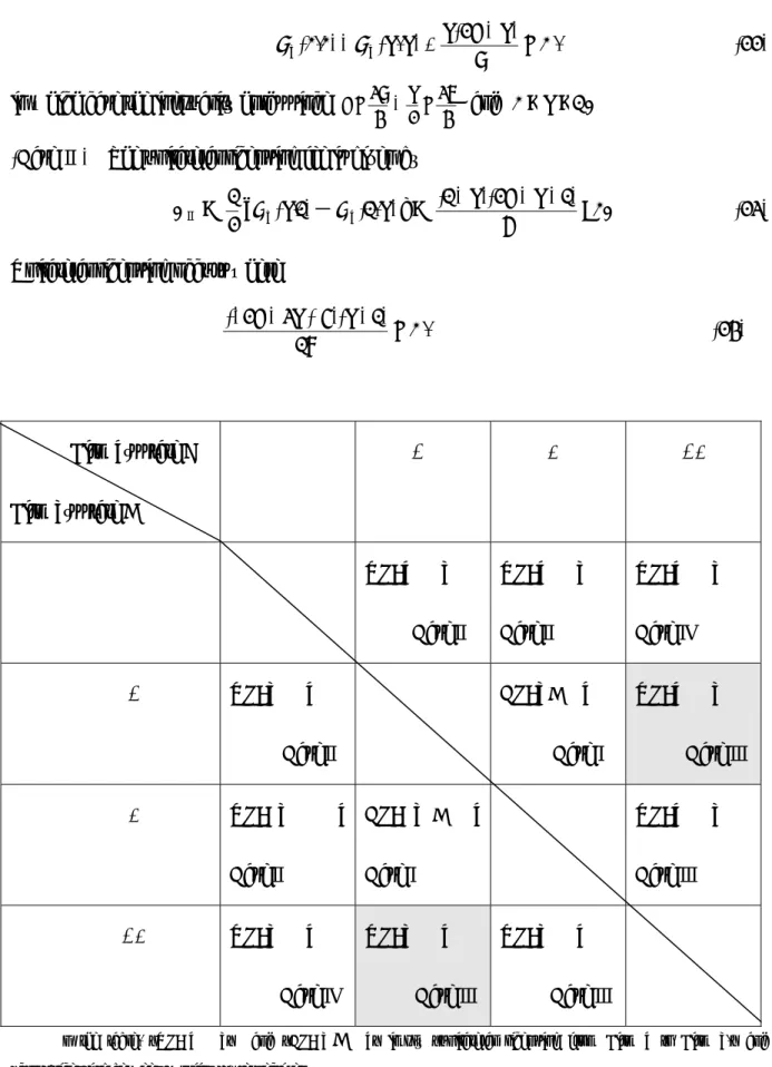
The state of nature of each firm depends on success(es) or failure(s) of the development of technologies. All cases where (cross-) licensing occurs are summarized in Table 1.
We classify the conditions under which (cross-) licensing occurs into four cases and derive the corresponding licensing fee in these cases.11
(Case Ⅰ) The cross-licensing fee is given by
FⅠ = 0. (21)
Cross-licensing occurs where
10 Both firms may agree to a licensing contract in which a licensee firm pays half the monopoly profit brought by producing at the lowered marginal cost realized by licensing, as the license fee in compensation for no production. The final gain of each firm after the side payment in this contract is, of course, larger than that where firms compete in a Cournot manner. However, the former is interpreted as an illegal act from the antitrust point of view. See the description in Section 3.2 and Example 4 in the Appendix of Antitrust Guidelines for
Collaborations Among Competitors (April 2000) issued by the Federal Trade Commission and the U. S. Department of Justice. They say that 'Agreements of a type that always tends to raise price or reduce output are per se illegal.' The contract in which the licensee firm produces the monopoly output and pays half the monopoly profit as a licensing fee to the licensor firm seems to be per se illegal. We thank Kuninobu Takeda, Associate Professor of Antitrust Law in Osaka University, for this justification of our assumption from the antitrust point of view and for the source of this citation. Hence, we assume that two firms compete in a Cournot manner after the licensing contract.
11 For the concrete derivation of the licensing conditions and the licensing fees in the case containing the four categories, see Appendix 2.
0 9 ) 2 ( ) , ( ) 0 , 0 ( − y k k = k a−k ≥ x π π , (22)
in which case the inequality holds since
4 37 2 4 39− ≥ ≥ k a and 0≤ k≤1. (Case Ⅱ) The unilateral licensing fee is given by
FⅡ = 2 1 [πx(k,1)−πy( k1, )] = 6 ) 1 2 )( 1 ( −k a−k− >0. (23) Unilateral licensing occurs where
0 18 ) 1 )( 5 3 2 (− a− k+ k− ≥ , (24)
Firm y’s state Y Firm x’s state X φ A B AB φ UL: y → x CaseⅡ UL: y → x CaseⅡ UL: y → x Case Ⅳ A UL: x → y CaseⅡ CL: x↔ y CaseⅠ UL: y → x Case Ⅲ B UL: x → y CaseⅡ CL: x ↔ y CaseⅠ UL: y → x Case Ⅲ AB UL: x → y Case Ⅳ UL: x → y Case Ⅲ UL: x → y Case Ⅲ
In the table, “UL: y →x” and “CL: x↔ y” imply “unilateral licensing from Firm y to Firm x,” and “cross-licensing between two firms,” respectively.
in which case the inequality holds since 4 37 2 4 39− ≥ ≥ k a and 0≤ k≤1. (Case Ⅲ) The unilateral licensing fee is given by
FⅢ= 2 1 [πx( k0, )−πy(k,0)] = − ≥ 6 ) 2 ( a k k 0. (25) Unilateral licensing occurs where
0 18 ) 5 2 ( ≥ − k a k , (26)
in which case, again, the inequality holds since
4 37 2 4 39− ≥ ≥ k a and 0≤ k≤1.
(Case Ⅳ) This case consists of two sub-cases in which unilateral licensing occurs. One sub-case is where only one technology is licensed. The other sub-case is where both technologies are licensed. As we show in Appendix 2, the strategy of unilateral licensing of both technologies is more beneficial for the licenser firm than that of licensing only one technology. We analyze this latter type of licensing. The unilateral licensing fee is given by
FⅣ= 2 1 [πx(0,1)−πy(1,0)]= 6 1 2a− >0. (27)
Unilateral licensing occurs where 0 18 5 2 > − a , (28)
in which case the inequalities in (27) and (28) hold because
4 37 2 4 39− ≥ ≥ k a .
Now, we are ready to derive the R&D investment game in duopoly with a (cross-) licensing system.
5. R&D investment with (cross-) licensing
Examining cells in Table 1 where (cross-) licensing occurs, we can express the case by using the realized marginal cost of firm i before (cross-) licensing as (( j) ci,cj). Then, we see that all the cases with (cross-) licensing are (k, k), (0, k), (0, 1), (k, 1), (k, 0), (1, 0) and (1,
(1) The firm i ’s profit realized in state (k, k) ( in this case, cross-licensing occurs and the licensing fee is zero) is
) ) 1 )( 1 ( ) 1 ( ) 1 (( xA xB yA yB xA xB yA yB kk i e e e e e e e e − − − − − − − − − + − − − = π πi(0,0). (29) (2) The firm i ’s profit realized in (0, k) is
= k i0 π (1−e−xA)(1−e−xB){e−yA +e−yB −2e−yAe−yB}[ (0,0) i π +FⅢ]. (30)
(3) The firm i ’s profit realized in (0, 1) is = 01 i π (1−e−xA)(1−e−xB)e−yAe−yB[ (0,0) i π +F ]. Ⅳ (31)
(4) The firm i ’s profit realized in (k, 1) is = 1 k i π [e−xA +e−xB −2e−xAe−xB]e−yAe−yB[ ( kk, ) i π +FⅡ]. (32)
(5) The firm i ’s profit realized in (k, 0) is = 0 k i π [e−xA +e−xB −2e−xAe−xB](1−e−yA)(1−e−yB) [ (0,0) i π -FⅢ]. (33)
(6) The firm i ’s profit realized in (1, 0) is = 10 i π e−xAe−xB (1−e−yA)(1−e−yB) [ (0,0) i π -F ]. Ⅳ (34)
(7) The firm i ’s profit realized in (1, k) is = k i 1 π e−xAe−xB (e−yA +e−yB −2e−yAe−yB) [ ( kk, ) i π -FⅡ]. (35)
Using the profits realized in states above, we express the expected profit of firm i as
i Π~ =Π +i CL i Π
{
} {
}
[
A k FⅢ B FⅣ]
e e xA − xB i − i + + i − i + − +(1 − )(1 − ) π (0,0) π (0, ) π (0,0) π (0,1){
} {
}
[
B k k k FⅡ C k FⅢ]
e e e e xA + xB − xA xB i − i + + i − i − +( − − 2 − − ) π ( , ) π ( ,1) π (0,0) π ( ,0){
} {
}
[
C FⅣ A k k k FⅡ]
e e xA xB i − i − + i − i − + − − π (0,0) π (1,0) π ( , ) π (1, ) (36)where A = e−yA +e−yB −2e−yAe−yB,B = e−yAe−yB ,C = (1−e−yA)(1−e−yB) (37) The increment to Firm i ’s expected profit associated only with cross-licensing CL
i Π is given by CL i Π = (1−e−xA)e−xB(1−e−yB)e−uAh+e−xA(1−e−xB)(1−e−yA)e−yBh, (38) where h =πi(0,0)−πi( kk, ).
Deriving the first-order condition and setting s= e−yA = e−yB = e−xA = e−xB, by using the fact that we derive the symmetric equilibrium, yields
B x A y B x A x e e e e s A x a k s − − − − = = = = ∂ Π ∂ ≡ Ω( , , ) ~ = B x A y B x A x B x A y B x A x e e e e s A CL e e e e s A x x = − =− = − =− ∂ =− = − =− = − Π ∂ + ∂ Π ∂ + )] ( ) ( )[ 1 2 ( )] ( ) ( )[ 1 ( s A n7 FⅢ B n8 FⅣ s s B n9 FⅡ C n1 FⅢ s − + + + + − + + − 0 )] ( ) ( [ 1 4 5 2 + − + − = −s C n n FⅣ A n FⅡ . (39)
After tedious calculations, we obtain the profit-maximization condition:12
0 1 ) 2 ( 6 1 ) 3 6 8 4 ( 18 1 ) 1 2 2 2 ( 9 1 ) , , ( = 2 − + − 4 + 2 − + − 2 + − − = Ω s k a k ak a s k ak a s k a k s (40)
From the l.h.s. of (40) we see that
. 144 151 72 1 ) 72 7 36 1 ( ) 2 151 7 2 ( 72 1 ) , , 2 1 ( =− 2 − − + = + − 2 − Ω k a k ak a k a k
As in the benchmark case, we assume that . 0 144 151 72 1 ) 72 7 36 1 ( ) , , 2 1 ( = + − 2 − > Ω k a k a k
This assumption implies that . 1 0 , 14 4 151 2 2 ≤ ≤ + + > k k k a (41)
Now, we need two lemmas to prepare for the result on equilibrium existence.
The two lemmas and their proofs and the proof of the following proposition are presented in Appendix 3.
From these two lemmas, we immediately obtain the following equilibrium existence result.
Proposition 2
Suppose that } 14 4 151 2 , 2 4 39 max{ 2 + + − > k k ka . Then there exists a positive symmetric equilibrium ) 2 1 , 0 ( ~∈
s in our model with (cross-) licensing.13
In any ) 2 1 , 0 ( ~s∈ , we have k s ∂ ∂~ < 0 and ~ <0 ∂ ∂ a s .
6. Effects of a (cross-) licensing system on R&D investment
In this section, we compare the equilibrium investment level without a (cross-) licensing
system with that with a (cross-) licensing system. The two lemmas needed for derivation of the
main result and their proofs are presented in Appendix 4. We also present the proof of the proposition in Appendix 4.
We establish the following proposition.
Proposition 3
(1) Suppose that the two technologies are not very partially complementary, such that 2
1
0≤k≤k** < . The licensing system discourages R&D investment, i.e.
2 1 ~ 0<s* <s < .
(2) Suppose that the two technologies are sufficiently partially complementary, such that
13 We can show that Ω(1,k,a)>(≤)0⇔∀k∈[0, k*]([k*, 1]),where 25 50 115. 5
1 2 *=a− a − a+
k Then, there
exists an s~~ such that ~~ 1 2
1< s < and Ω(s~~,k,a)=0, for k∈[k*,1]. We also show, as we do in footnote 6, that ~~s( ~~ 1
2
1< s< ) never satisfies the second-order condition. By Kuhn–Tucker conditions, in this case, there exists equilibrium~ =s 1. It implies, however that each firm does not invest at all at the equilibrium. This case is not interesting and is omitted.
1 2
1
*
* < <k ≤
k and there exist any points ) 2 1 , 0 ( 0 ∈ s such that φ(s0,k,a)=Ω(s0,k,a). (2-a) If there exists a unique )
2 1 , 0 ( 0 ∈
s such that φ(s0,k,a)=Ω(s0,k,a)>0, the licensing system discourages R&D investment, i.e.
2 1 ~ 0<s*<s < . (2-b) If there exists a unique )
2 1 , 0 ( 0 ∈
s such that φ(s0,k,a)=Ω(s0,k,a)<0, the licensing system encourages R&D investment, i.e.
2 1 ~
0<s <s*< . (2-c) If there exists a unique )
2 1 , 0 ( 0 ∈
s such that φ(s0,k,a)=Ω(s0,k,a)=0, the licensing system is neutral for R&D investment, i.e.
2 1 ~
0<s =s* < .
We give some numerical examples for this proposition. See Figure 2 for (1), Figure 3 for (2-b) and Figure 4 for (2-a).
[Insert Figure 2, Figure 3 and Figure 4 here]
We explain intuitively the discouragement to R&D investment result. From (38) the increment to firm i ’s expected profit with only cross-licensing CL
i Π is given by CL i Π = (1−e−xA)e−xBe−yA(1−e−yB)h+e−xA(1−e−xB)(1−e−yA)e−yBh, where h = 0 9 ) 2 ( ) , ( ) 0 , 0 ( − y k k = k a−k ≥ x π π .(Q(22)) (42)
The partial derivative term of CL i
π evaluated at the symmetric equilibrium (s =e−xA =e−xB =e−yA =e−yB) is given by the following expression.
0 ) 1 )( 1 2 ( 9 1 ) , , ( = 2 − − < = ∂ Π ∂ − − − − = = = = h s s s a k s M xA s e xA exB e yA e yB CL (43)
However, from Proposition 2, we see that ) 2 1 ( ~
0< s < at equilibrium. The expression above shows that the existence of cross-licensing discourages R&D investment. On the other
hand, the increment to firm i’s expected profit resulting from unilateral licensing is given by the following formula:
, ) 1 ( ) 1 ( ) 1 ( ) 1 ( ) 1 )( 1 )( 1 ( ) 1 ( ) 1 )( 1 ( ) 1 )( 1 ( ) 1 ( ) 1 )( 1 )( 1 ( ) 1 )( 1 ( ) 1 )( 1 ( Ⅱ Ⅱ Ⅱ Ⅱ Ⅲ Ⅲ Ⅲ Ⅲ Ⅳ Ⅳ π π π π π π π π π π B A B A B A B A B A B A B A B A B A B A B A B A B A B A B A B A B A B A B A B A y y x x y y x x y y x x y y x x y y x x y y x x y y x x y y x x y y x x y y x x UL e e e e e e e e e e e e e e e e e e e e e e e e e e e e e e e e e e e e e e e e − − − − − − − − − − − − − − − − − − − − − − − − − − − − − − − − − − − − − − − − − + − + − + − + − − − + − − − + − − − + − − − + − − + − − = Π where . ) , 1 ( ) , ( ) 1 , ( ) , ( , ) 0 , ( ) 0 , 0 ( ) , 0 ( ) 0 , 0 ( , ) 0 , 1 ( ) 0 , 0 ( ) 1 , 0 ( ) 0 , 0 ( Ⅱ Ⅱ Ⅱ Ⅲ Ⅲ Ⅲ Ⅳ Ⅳ Ⅳ F k k k F k k k F k F k F F x x x x x x x x x x x x − − = + − ≡ − − = + − ≡ − − = + − ≡ π π π π π π π π π π π π π π π
From the corresponding part of the first-order condition of the symmetric equilibrium (s =e−xA =e−xB =e−yA =e−yB) is given by the following expression.
Ⅱ Ⅲ Ⅳ Ⅱ Ⅱ Ⅲ Ⅲ Ⅳ Ⅱ Ⅱ Ⅱ Ⅱ Ⅲ Ⅲ Ⅲ Ⅲ Ⅳ Ⅳ π π π π π π π π π π π π π π π π π π ) 3 ~ 4 ( ~ ) 1 ~ 4 ( ) ~ 1 ( ~ ) 1 ~ 2 )( ~ 1 ( ~ ) ~ 1 ( ~ 2 ) 1 ~ 2 ( ~ ) 1 ~ 2 ( ) ~ 1 ( ~ ) ~ 1 ( ~ 2 ) 1 ~ 2 )( ~ 1 ( ~ ) 1 ( ) 1 ( ) 1 ( ) 1 )( 1 )( 1 ( ) 1 ( ) 1 ( ) 1 )( 1 ( ) 1 )( 1 ( ) 1 )( 1 ( ) 1 ( 3 2 2 3 3 2 2 2 2 ~ − + − − + − − = − − − + − − + − + − − = − − − − − − + − − − − − − + − − + − − + − − − − = ∂ Π ∂ − − − − − − − − − − − − − − − − − − − − − − − − − − − − − − − − − − − − − − − − s s s s s s s s s s s s s s s s s s s s e e e e e e e e e e e e e e e e e e e e e e e e e e e e e e e e e e e e e e e e x B A B A B A B A B A B A B A B A B A B A B A B A B A B A B A B A B A B A B A B A y y x x y y x x y y x x y y x x y y x x y y x x y y x x y y x x y y x x y y x x s A UL (44)
From (23), (25), (27) and the definitions of πⅡ, πⅢ, πⅣ above, we obtain
. 18 5 2 , 18 ) 5 2 ( , 18 ) 5 3 2 )( 1 ( − = − = − + − = k a k Ⅲ k a k Ⅳ a Ⅱ π π π (45)
Calculating the partial derivatives of πⅡ, πⅢ, πⅣ w.r.t. aand k in (45) yields
. 4 37 , 1 0 , 0 , 0 9 5 , 0 18 2 6 8 1 0 , 0 9 1 , 0 9 , 0 9 1 > ≤ ≤ = ∂ ∂ ≥ − = ∂ ∂ < − − = ∂ ∂ ≤ ≤ > = ∂ ∂ ≥ = ∂ ∂ ≥ − = ∂ ∂ a k k k a k a k k k a k a k a Ⅳ Ⅲ Ⅱ Ⅳ Ⅲ Ⅱ π π π π π π
At the symmetric equilibrium ) 2 1 ( ~
Ⅲ Ⅲ Ⅲ π π π 2 2(1 ~) ~ 2 ) 1 )( 1 ( ) 1 )( 1 ( s s e e e e e e e e xA xB yA yB xA xB yA yB − = − − + − − − − − − − − − − (46)
work in the same direction to increase R&D investment (shift the function Ω upward). These two terms are the marginal benefit to firm x when it slightly increases investment in development of technology A in the cases {AB, A} and {A, AB}, respectively (which correspond to the two shaded cells in Table 1). In these two cases, the increase of xA is always beneficial to firm x since it succeeds in developing technology A. However, all the other eight terms in (44) work to shrink R&D investment (shift the function Ω downward). In these cases, although the increase of xA brings firm x a positive marginal benefit if it succeeds in developing technology A (for example, see the corresponding cell to the case Ⅳ{AB,φ} in Table 1), at the same time it brings a negative marginal benefit since the expected benefit as a unilateral licensee of technology A from firm y decreases in the pair case where firm x fails to develop technology A (See the UL cells to case Ⅳ{φ, AB} in Table 1). The corresponding part of the first-order condition of the increment to firm i ’s expected profit with only cross-licensing CL
i
Π also works to shrink R&D investment (shift the function Ω downward). The total negative effect dominates in most cases when the underlying market demand for the product ais sufficiently large, since πⅡ, πⅢ, πⅣ are
nondecreasing in a. In some cases, however, the positive effects dominate. If the extent of complementarity k∈[0,1] is so large and the underlying demand a is small enough, these cases tend to occur.
To explain these results intuitively, note that we normalize the reduction of the marginal cost of production associated with the R&D development to unity. The underlying demand a
is also looked upon as reduced to unity (a is the original market size divided by the amount of marginal cost reduction). Thus, the change in a is incomparably larger than the change of
Let us focus on the comparative statics w.r.t. k when the underlying demand a is small enough and the magnitude of the marginal cost reduction is large compared with the underlying demand. From the above definitions, πⅡ, πⅢ, πⅣ and h represent the ex
post profit of each firm under unilateral licensing of only one technology where the licensee has not developed any technology, the ex post profit of the firm under unilateral licensing of one technology by the licensor who has developed both technologies and the licensee has developed only one technology, the ex post profit of the firm under unilateral licensing of two developed technologies where the licensee has no developed technologies, and the incremental profit of each firm under cross-licensing, respectively. As the extent of the complementarity k increases, πⅢ and h increase while πⅣ does not change and πⅡ
decreases. Therefore, when k is large but a is small enough, the positive effect (associated with πⅢ) presented in (46) dominates the total negative effects associated with terms πⅡ in
(44) and h (given by (43)).
This proposition shows that a (cross-) licensing system promotes R&D investment in some cases when the duopolistic firms produce goods by using two partially complementary technologies. In these cases, the extent of complementarity k is sufficiently large and the underlying demand a is small enough.
Okamura, Shinkai and Tanaka (2002) established that the existence of a cross-licensing system always discourages firm’s R&D investments, when the duopolistic firms produce a good by using the two completely complementary technologies. In their model, no unilateral licensing can occur since firms require both technologies to produce the good. The existence of a cross-licensing system decreases firms’ incentives for R&D through the chance to exchange their technologies. As we have shown in this paper, however, unilateral licensing may encourage firms’ incentives for R&D through the chance of their receiving (paying) the licensing fee when the extent of complementarity k is sufficiently large and the underlying demand a is small enough. When two not quite completely complementary technological
innovations occur, this positive effect of unilateral licensing on firms’ incentives for R&D may surpass the negative effect of cross-licensing upon their incentives.
7. Welfare comparison at the equilibria with and without licensing
In this section, we compare economic welfare evaluated at the equilibria, s and *
s~with and without (cross-) licensing. Since we see that we cannot derive two equilibrium solutions s and * s~ analytically from the discussion in the preceding section, so comparison
of economic welfare at s and * s~ is conducted for the numerical solutions s ’s and * s~’s
presented in preceding section in three cases in the preceding section, where a = 15, k = 0.3, where a = 9.5, k = 0.95 and where a = 15, k = 0.95.
Set * * * * * ( * * ln *) s x x e e e e s = −xA = −xB = −yA = −yB A = B =− in (6) and multiply it by 2, we define the expected producers’ surplus at the symmetric equilibrium without licensing as
, ln 4 ) , , ( 2 ) , , ( ) 1 ( 4 ) , , ( ) 1 ( 2 ) , , ( * * 4 2 * * 2 * * * 1 2 * * * s k a s H s k a s s H s k a s H s k a s EPS ≡ − + − + + (47) where 4H (s*,a,k),i=1,2,
i implies Hi,i=1,2,4given by (7a), (7b) and (7d) evaluated at
* * * *
* e xA e xB e yA e yB
s = − = − = − = − . That is, we have ) , , ( * 1 s k a H = (1−s*)2 (0,0) x π + )2s*(1−s* ( k0, ) x π + *2 (0,1) x s π , (48a) ) , , ( * 2 s k a H = (1−s*)2 (k,0) x π + )2s*(1−s* ( kk, ) x π +s*2 (k,1) x π , (48b) ) , , ( * 4 s k a H = (1−s*)2 (1,0) x π + )2s*(1−s* ( k1, ) x π + *2 (1,1) x s π . (48c)
We know well that the consumers’ surplus in the Cournot equilibrium of our setting is
given by ( , ) , 2 1 )) , ( ( 2 y x y x c Q c c c Q CS = where Q(cx,cy)=qx(cx,cy)+qy(cy +cx).
Replacing )πx(cx,cy by ))CS(Q(cx,cy in (48a), (48b) and (48c), we define the expected consumers’ surplus as
), , , ( 2 ) , , ( ) 1 ( 4 ) , , ( ) 1 ( 2 ) , , ( * 4 2 * * 2 * * * 1 2 * * * s k a s J s k a s s J s k a s J s k a ECS ≡ − + − + (49) where ) , , ( * 1 s k a J = (1−s*)2 CS(Q(0,0))+2s*(1−s*)CS(Q(0,k))+s*2CS(Q(0,1)), (50a) ) , , ( * 2 s k a J = (1−s*)2 CS( kQ( ,0))+2s*(1−s*)CS(Q(k,k))+s*2CS(Q(k,1)), (50b) ) , , ( * 4 s k a J = (1−s*)2 CS(Q(1,0))+ )2s*(1−s* CS(Q(1,k))+s*2CS(Q(1,1)). (50c)
Accordingly, the expected social surplus at the symmetric equilibrium without licensing is defined as ) , , ( ) , , ( ) , , ( * * * * * * s k a EPS s k a ECS s k a ESS = + . (51)
From Table 1 and the description following Table 1, the expect profit of firm x at the equilibrium with (cross-) licensing is given by
, ) 1 ( ) 1 ( ) 1 )( 1 ( x x 1 x x 2 x x 3 x x 4 A B WL x ≡ −e A −e B L + −e A e BL +e A −e B L +e Ae AL −x −x Π − − − − − − − − (52) where ], ) 0 , 0 ( [ ] ) 0 , 0 ( )[ 1 ( ] ) 0 , 0 ( [ ) 1 ( ) 0 , 0 ( ) 1 )( 1 ( 1 Ⅳ Ⅲ Ⅲ e e F F e e F e e e e L x y y x y y x y y x y y A A B A B A B A + + + − + + − + − − = − − − − − − − − π π π π (53a) ], ) , ( [ ) 0 , 0 ( ) 1 ( ) , ( ) 1 ( ] ) 0 , 0 ( )[ 1 )( 1 ( 2 Ⅱ Ⅲ e e k k F e e k k e e F e e L x y y x y y x y y x y y A A B A B A B A + + − + − + − − − = − − − − − − − − π π π π (53b) ], ) , ( [ ) , ( ) 1 ( ) 0 , 0 ( ) 1 ( ] ) 0 , 0 ( )[ 1 )( 1 ( 3 Ⅱ Ⅲ e e k k F k k e e e e F e e L x y y x y y x y y x y y A A B A B A B A + + − + − + − − − = − − − − − − − − π π π π (53c) ). 1 , 1 ( ] ) , ( )[ 1 ( ] ) , ( [ ) 1 ( ] ) 0 , 0 ( )[ 1 )( 1 ( 4 x y y x y y x y y x y y A A B A B A B A e e F k k e e F k k e e F e e L π π π π − − − − − − − − + − − + − − + − − − = Ⅱ Ⅱ Ⅳ (53d)
Similarly, we can obtain the expect profit of firm y at the equilibrium. Setting ) ~ ln ~ ~ ( ~ B A ~ ~ ~ ~ B A B A e e e x x s e
s = −x = −x = −y = −y = =− in these expected profits, and taking into
consideration that all license fee terms cancel out at the equilibrium. Then, we can obtain the expected producers’ surplus at the symmetric equilibrium with licensing as
s a s k a s s s a s s s s k k s s s s s a k s EPSWL x x x ~ ln 4 9 ) 1 ( ~ 2 9 ) ( ) ~ 1 )( ~ 1 ( ~ 4 9 ) ~ 1 ( ) ~ 1 ( 2 ~ ln 4 ) 1 , 1 ( ~ 2 ) , ( ) ~ 1 )( ~ 1 ( ~ 4 ) 0 , 0 ( ) ~ 1 ( ) ~ 1 ( 2 ) , , ~ ( 2 4 2 2 2 2 2 4 2 2 2 + − ⋅ + − ⋅ + − + ⋅ + − = + ⋅ + ⋅ + − + ⋅ + − ≡ π π π (54) Similar toEPSWL(~s,k,a), we also define the expected consumers’ surplus as
. 9 ) 1 ( 2 ~ 9 ) ( 2 ) ~ 1 )( ~ 1 ( ~ 2 9 2 ) ~ 1 ( ) ~ 1 ( )) 1 , 1 (( ( ~ )) , ( ( ) ~ 1 )( ~ 1 ( ~ 2 )) 0 , 0 ( ( ) ~ 1 ( ) ~ 1 ( ) , , ~ ( 2 4 2 2 2 2 2 4 2 2 2 − ⋅ + − ⋅ + − + ⋅ + − = ⋅ + ⋅ + − + ⋅ + − ≡ a s k a s s s a s s Q CS s k k Q CS s s s Q CS s s a k s ECSWL (55) The expected social surplus at the symmetric equilibrium with licensing is defined as
) , , ~ ( ) , , ~ ( ) , , ~ (s k a EPS s k a ECS s k a ESSWL = WL + WL . (56)
To compare economic welfare evaluated at the equilibria s and * s~with and without
(cross-) licensing, solved numerically in three cases where a = 15, k = 0.3, where a = 9.5, k = 0.95 and where a = 15, k = 0.95), we calculate
) , , ~ ( ), , , ~ ( ), , , ( ), , , ( ), , , ( * * * * *
* s k a ECS s k a ESS s k a EPS s k a ECS s k a
EPS WL WL and ) , , ~ (s k a
ESSWL in these cases. Denote the variations of the expected producers’, consumers’
and social surplus by ∆PS =EPSWL−EPS*, ∆CS =ECSWL −ECS* and *
ESS ESS
SS = WL −
∆ .
(i) Where a = 15, k = 0.3, the two equilibria are s* =0.35384 and
37943 . 0
~ =s (Figure 2). From (47),(49),(51),(54),(56) and (56) we have , 502 45. ) 15 , 3 . 0 , 0.37943 ( 219 . 44 ) 15 , 3 . 0 , 0.35384 ( * = <EPSWL = EPS (57a) 378, 49. ) 15 , 3 . 0 , 0.37943 ( 277 48. ) 15 , 3 . 0 , 0.35384 ( * = < ECSWL = ECS (57b) 88 94. ) 15 , 3 . 0 , 0.37943 ( 496 92. ) 15 , 3 . 0 , 0.35384 ( * = < ESSWL = ESS . (57c)