JAIST Repository: 知識発見処理における欠損値を含むデータを処理するための効果的なアルゴリズムの研究

全文

(1)JAIST Repository https://dspace.jaist.ac.jp/. Title. 知識発見処理における欠損値を含むデータを処理するための効果的なアルゴリズムの研究. Author(s). 冨士川, 義和. Citation Issue Date. 2001-03. Type. Thesis or Dissertation. Text version. author. URL. http://hdl.handle.net/10119/746. Rights Description. Supervisor:HoTu Bao, 知識科学研究科, 修士. Japan Advanced Institute of Science and Technology.

(2) Efficient Algorithms for Dealing with Missing values in Knowledge Discovery. By Yoshikazu Fujikawa. A thesis submitted to School of Knowledge Science, Japan Advanced Institute of Science and Technology in partial fulfillment of the requirements for the degree of Master of Knowledge Science Graduate Program in Knowledge Science. Written under the direction of Professor Tu Bao Ho February 13, 2001. Copyright _ 2001 by Yoshikazu Fujikawa. i.

(3) Contents. Chapter 1 １１ Introduction 1.1 The missing value problem in KDD ------------------------------------ 1 1.2 Background --------------------------------------------------------------------1.3 Motivation and objectives 1.4 Approach and results. 2. --------------------------------------------------. 2. -------------------------------------------------------- 3. 1.5 Organization of this thesis. -------------------------------------------------. 3. Chapter 2 4 The missing value problem in KDD 2.1 The KDD process. -------------------------------------------------------------. 2.2 Targets of data mining. 4. ------------------------------------------------------. 6. 2.3 Standard form. ------------------------------------------------------------------. 6. 2.4 Missing values. ----------------------------------------------------------------- 7. 2.5 What is missing value problem? ------------------------------------------ 8 2.6 The methods to deal with missing values. ------------------------------. 9. Chapter 3 10 Investigation of algorithms to deal with missing values 3.1 Classification of missing values cases --------------------------------- 10 3.2 Methods for dealing with missing values. ---------------------------- 13. 3.2.1 Statistical methods ----------------------------------------------------. 14. 3.2.2 Machine learning methods ------------------------------------------ 15 3.2.3 Embedded methods ----------------------------------------------------. i. 18.

(4) 3.3 Evaluation. ---------------------------------------------------------------------. 3.3.1 Theoretical evaluation. ------------------------------------------------ 20. 3.3.2 Experimental comparative evaluation 3.3.2.1 Methodology. 19. ---------------------------. 22. ----------------------------------------------------. 22. 3.3.2.2 Results on datasets with symbolic attributes -------- 23 3.3.2.3 Results on datasets with numeric attributes ---------. 25. 3.3.2.4 Results on datasets with mixed attributes ------------. 27. Chapter 4 30 Efficient algorithms to deal with missing values 4.1 Basic idea of scalable algorithms 4.2 Proposed Algorithms. ----------------------------------------. 30. ---------------------------------------------------------. 31. 4.2.1 Natural Cluster Based Mean and Mode method (NCBMM) -- 31 4.2.2 Distanced Cluster Based Mean and Mode method (DCBMM) ----- 32 4.2.3 k-Means Clustering Based Mean and Mode method (KMCMM) ----- 33 4.3 Evaluation. -----------------------------------------------------------------------. 4.3.1 Methodology. 35. ---------------------------------------------------------------. 4.3.2 Analysis of results. 35. -------------------------------------------------------- 37. 4.3.2.1 Error rate --------------------------------------------------------4.3.2.2 Execute time for replacing. -----------------------------------. 4.3.3 Experiment on census-income data set. 37 48. ---------------------------- 49. Chapter 5 50 Conclusion and future works 5.1 Comparing the methods -----------------------------------------------------5.2 Scalable algorithms to deal with missing values. --------------------. 50. 50. 5.3 Future works -------------------------------------------------------------------- 51. ii.

(5) List of Figures 2-1: The outline of KDD process. ------------------------------------------------------------. 2-2: Example of a dataset in standard form. 5. --------------------------------------------- 7. 3-1: Three cases of missing values in a data set. --------------------------------------- 11. 3-2: A result of our missing values case visualization program ------------------. 12. 3-3: Algorithm for replacement under same standard deviation ----------------- 15 3-4: Algorithm for mean and mode method --------------------------------------------- 15 3-5: Algorithm for nearest neighbor estimator. ----------------------------------------. 3-6: Algorithm for autoassociative neural network 3-7: Algorithm for decision tree imputation. 16. ---------------------------------- 17. --------------------------------------------. 18. 3-8: Comparing methods by error rates on led data set -----------------------------. 24. 3-9: Comparing methods by error rates on vot data set -----------------------------. 24. 3-10: Comparing methods by error rates on dna data set --------------------------. 24. 3-11: Comparing methods by error rates on wav data set --------------------------. 26. 3-12: Comparing methods by error rates on bld data set ---------------------------. 26. 3-13: Comparing methods by error rates on pid data set ---------------------------. 26. 3-14: Comparing methods by error rates on hea data set --------------------------. 28. 3-15: Comparing methods by error rates on smo data set --------------------------. 28. 3-16: Comparing methods by error rates on tae data set ---------------------------. 28. 4-1: Algorithm NCBMM. ----------------------------------------------------------------------. 31. 4-2: Algorithm RCBMM ----------------------------------------------------------------------. 32. 4-3: Algorithm KMCMM. 34. ---------------------------------------------------------------------. 4-4: Algorithm for k-means clustering. --------------------------------------------------- 35. 4-5: Error rates of each method with C4.5 classifier on mixed data sets ------. iii. 38.

(6) 4-6: Error rates of each method with C4.5 classifier on numeric data sets --4-7: Error rates of each method with C4.5 classifier on symbolic data sets ---. 39 40. 4-8: Error rates of each method with Na ve Bayesian classifier on mixed data sets ----. 41. 4-9: Error rates of each method with Na ve Bayesian classifier on numeric data sets ----- 42 4-10: Error rates of each method with Na ve Bayesian classifier on symbolic data sets ----- 43 4-11: Error rates of each method with k-nearest neighbor classifier on mixed data sets ----- 44 4-12: Error rates of each method with k-nearest neighbor classifier on numeric data set ---- 45 4-13: Error rates of each method with k-nearest neighbor classifier on symbolic data set ---- 46. iv.

(7) List of Tables 3-1: Methods for dealing with missing values. -----------------------------------------. 3-2: Theoretical evaluation of methods for dealing with missing values. ------. 14. 21. 3-3: Parameters of data sets ----------------------------------------------------------------- 22 3-4: Error rates on the datasets with symbolic attributes --------------------------. 23. 3-5: Error rates on the datasets with numeric attributes --------------------------. 25. 3-6: Error rates on the datasets with mixed attributes -----------------------------. 27. 4-1: Data set those have missing values on both numeric and symbolic attributes ----- 36 4-2: Data sets whose have missing values on numeric attributes ---------------. 36. 4-3: Data sets whose have missing values on symbolic attributes ---------------. 37. 4-4: Errors rate with C4.5 classifier on mixed data sets ---------------------------- 38 4-5: Errors rate with C4.5 classifier on numeric data sets ------------------------- 39 4-6: Errors rate with C4.5 classifier on symbolic data sets ------------------------. 40. 4-7: Error rates with Na ve Bayesian classifier on mixed data sets ------------- 41 4-8: Error rates with Na ve Bayesian classifier on numeric data sets ----------. 42. 4-9: Error rates with Na ve Bayesian classifier on symbolic data sets ---------. 43. 4-10: Error rates with k-nearest neighbor classifier on mixed data sets ------. 44. 4-11: Error rates with k-nearest neighbor classifier on numeric data sets ----. 45. 4-12: Error rates with k-nearest neighbor classifier on symbolic data sets ---. 46. 4-13: The order of methods for dealing with missing values on numeric attributes ----- 47 4-14: The order of methods for dealing with missing values on symbolic attributes ----- 47 4-15: Execute time for replacing on mixed data sets --------------------------------. v. 48.

(8) 4-16: Execute time for replacing on numeric data sets ----------------------------4-17: Execute time for replacing on symbolic data sets -----------------------------. 48 49. 4-18: Comparing replaced methods and direct processing method -------------- 49. vi.

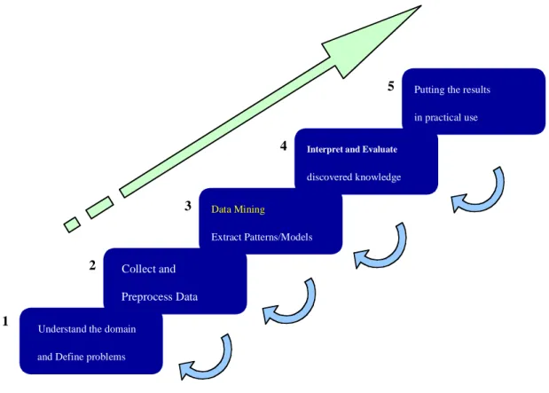
(9) Chapter 1 Introduction. 1.1. The missing value problem in KDD. The amount of data in the world, in our lives, seems to go on and increasing. The current progress of processing ability and memory capacity of computer enable to deal with more data. Knowledge Discovery in Databases (KDD) is the automatic extraction of non-obvious, hidden knowledge from large volumes of data. KDD has become a new area that attracts not only theoretical researchers but also practitioners. The KDD process consists of five phases [Mannila, 1996]: (1) Understand the domain and define problems, (2) Collect and preprocess data, (3) Extract patterns or models, (4) Interpret and evaluate discovered knowledge, (5) Putting the results in practical use. The third phase is called the data mining phase. It is the main part of KDD. In practice, most of effort and cost are occupied by the second phase. One hard problem of KDD is the occurrence of missing values in data sets. This problem occurs when certain values in the data sets are not observed in the phase of data collection. Missing values may hide a true answer underlying in the data, and many data mining programs used in the third phase cannot be applied to data that includes missing values. Many methods to deal with missing values have been developed so far.. 1.

(10) 1.2. Background. There are some kinds of methods to deal with missing values [Liu, 1997]. The simplest way is to ignore the instances containing unknown values. Another kind of methods for dealing with missing values is to try to determine these values using other information. Kononenko et al. [1984] used class information to estimate missing values. Another method suggested by Shapiro and described by Quinlan [1986] is to use a decision tree approach to decide the missing values of an attribute. We describe its detail in section 2 of chapter 3. Quinlan [1986] and Breiman [1984] use other methods specialized for their decision tree data mining tools, C4.5 and CART respectively. Dynamic path generation method proposed by White [1987] and Lazy decision tree method proposed by Friedman et al. [1996] are other methods to deal with missing values flexibly. They are used in testing phase in tree classifying methods.. 1. 3 Motivation and objectives As we described in previous section, many methods to deal with missing values have been developed. But it is still not clear how different methods can be appropriately used in a given application. Especially, one critical problem is how to deal with missing values in a huge data set. We must think of scalable methods for such a data set. Therefore, the objectives of our study are: 1.. to investigate several well-known methods of processing missing values in KDD by theoretical and experimental comparative evaluation;. 2.. to find scalable algorithms to deal with missing values for huge datasets in data mining.. 2.

(11) 1.4 Approach and results Our approach is cluster-based filling up missing values with simple clustering algorithms for large datasets. These methods are simple and take less computation cost than many ones. By experimental comparison on large datasets, it is shown that they achieve high quality filled up datasets which are comparable to that obtained by complicated methods. Moreover, they are much faster than others. In our information age, the methods that take high computation cost are neither scalable nor realistic. Our methods are useful and make accurate results even for large datasets.. 1.5 Organization of this thesis This thesis is organized as follows. In chapter 2, we introduce to the KDD process, the standard form of datasets used in KDD and missing value problem. In chapter 3, we summarize different possible cases of missing values in datasets and an investigation of popular existing methods for dealing with missing values in theoretical and practical views. In chapter 4, we describe our new algorithms and results of the experiment to compare methods for dealing with missing values. In chapter 5, we give the conclusion and future research.. 3.

(12) Chapter 2 The missing value problem in KDD. 2.1 The KDD process The goal of knowledge discovery is to obtain useful knowledge from large collections of data. Such a task is inherently interactive and iterative: one cannot expect to obtain useful knowledge simply by pushing a lot of data to a black box. The user of a KDD system has to have a solid understanding of the domain in order to select the right subsets of data, suitable classes of patterns, and good criteria for interestingness of the patterns. Thus KDD systems should be seen as interactive tools, not as automatic analysis systems. As described in the previous chapter, the KDD process contains five phases (Fig. 2-1); (1) understand the domain and define problems, (2) collect and preprocess data, (3) extract patterns or models, (4) interpret and evaluate discovered knowledge and (5) putting the results in practical use. KDD is not only straightforward process but inherently interactive and iterative. Understanding the domain of the data is naturally a prerequisite for extracting anything useful: the user of a KDD system has to have some sort of understanding about the application area before any valuable information can be obtained. Other words, if the user wants to extract some useful knowledge from the data, he must know about structure and features of the domain. And he must what kind of knowledge he needs concretely. Preparation of the data set involves selection of the data sources, integration of heterogeneous data, cleaning the data from errors, assessing noise, dealing with missing values, etc. This step can easily take up to 80% of the time needs for the whole KDD process.. 4.

(13) 5. Putting the results in practical use. 4. Interpret and Evaluate. discovered knowledge. 3. Data Mining Extract Patterns/Models. 2. Collect and Preprocess Data. 1. Understand the domain and Define problems. Fig. 2-1: The outline of KDD process. This is not surprising, since the difficulties in data integration are well known. The pattern discovery phase in KDD is the step where the interesting and frequently occurring patterns are discovered from the data. The data mining step can use various techniques from statistics and machine learning, such as rule learning, decision tree induction, clustering, inductive logic programming, etc. The emphasis in data mining research is mostly on efficient discovery of fairly simple patterns. The KDD process does not stop when patterns have been discovered. The user has to be able to understand what has been discovered, to view the data and patterns simultaneously, contrast the discovered patterns with background knowledge, etc. Postprocessing of discovered knowledge involves steps such as further selection or ordering of patterns, visualization, etc. Some approaches to KDD methodology put a heavy emphasis on postprocessing. The KDD process is necessarily iterative: the results of a data mining step can show that some changes should be made to the data set formation step, post-processing of patterns can cause the user to look for some slightly modified types of patterns, etc. Efficient support for. 5.

(14) such iteration is one important development topic in KDD.. 2.2 The target of data mining Data mining functionalities are used to specify the kind of patterns to be found in data mining tasks. In general, data mining tasks can be classified into two categories: descriptive and predictive. Descriptive mining tasks characterize the general properties of the data in the database. Predictive mining are association analysis, classification/prediction and clustering. Association analysis is the discovery of association rules showing attribute-value conditions that occur frequently together on a given set of data. Basket analysis is used for several areas. Classification is the process of finding a set of models (or functions) that describe and distinguish data classes or concepts, for the purpose of being able to use the model to predict the class of objects whose class label is unknown. Decision trees and neural networks are used for this task. Classification can also be used to predict a class label of a new instance. Clustering analyzes data objects without consulting a known class label. In this paper, we discuss about how to deal with missing values for classification/prediction tasks.. 2.3 Standard form In the real world of data mining applications, more effort is expended preparing data than applying a prediction program to data. Prediction programs look at data in a mechanical way. They expect the data to be specified in a standard form. Given this form, they search a space of possibilities in a very comprehensive way, far exceeding human capabilities. The concept of a standard form is more than simple formatting of data. A standard form helps to understand the advantages and limitations of different prediction techniques and how they reason with data. Standard form is made into a format of spreadsheet. The rows of the standardized data represent units, also called cases, instances, observations, or subjects depending on context,. 6.

(15) and the columns represent variables measured for each unit. Usually, each unit has several descriptive attribute and one class attribute. The entries in a data matrix are real numbers, representing the values of essentially continuous variables, such as age and income, or representing categories of response, which may be ordered (e.g., level of education) or unordered (e.g., race and sex). Often, Boolean values that are represented as 1 or 0 for meaning true or false respectively are used. We show the example of a dataset in standard form in Fig. 2-2.. ... 10,M,SUBACUTE,37,15,-,6000,2,abnormal,-,2852,F,-,multiple,?,2137,n,ABSCESS,VIRUS 12,M,ACUTE,38.5,15,-,10700,4,normal,+,1080,F,-,ABPC+CZX,?,70,n,BACTERIA,BACTERIA 15,M,ACUTE,39.3,15,-,6000,0,normal,+,1124,F,-,FMOX+AMK,?,48,n,BACTE(E),BACTERIA 16,M,SUBACUTE,38,15,+,12600,4,abnormal,+,41,F,-,ABPC+CZX,?,?,n,ABSCESS,VIRUS .... Fig. 2-2: Example of a dataset in standard form. 2.4 Missing values Missing values are values of instances that are not observed. Most datasets encountered in practice contain missing values. It is occurred in the phase of data collecting. Why do missing values occur? For example, respondents in a household survey may refuse to report income. In an industrial experiment some results are missing because of mechanical breakdowns unrelated to the experimental process. In an opinion survey some individuals may be unable to express a preference for one candidate over another. In the first two examples it is natural to treat the values that are not observed as missing, in the sense that there are true underlying values that would have been observed if survey techniques had been better or the industrial equipment had been better maintained. In the third example, however, it is less clear that a well-defined candidate preference has been masked by the nonresponse; thus it is less natural to treat the unobserved values as missing. Instead, the lack of a response. 7.

(16) is essentially an additional point in the sample space of the variable being measured, which identifies a don t know stratum of the population [Little, 1987]. Roughly, we can classify the reason why missing values occur. One is that the values are out of expected range. Another is simple reason that are some errors occurred on data entry, for example, operator s mistakes, computer s breakdown and so on.. 2.5 What is the missing value problem? One hard problem of KDD is the occurrence of missing values in data sets. They may hide a true answer underlying in the data; a missing value cannot be multiplied or compared. Most of prediction methods used in the data mining phase can t deal with data that includes missing values. Neither many statistical data mining techniques, nor nearest neighbor classifier, na ve bayes classifier, etc. can deal with the dataset with missing values. Moreover, the data mining methods, those can deal with missing values are disturbed from effective data mining processing somewhat. Some data mining methods, based on the technique of a decision tree, C4.5 and CART handle missing values by the kind of build in approaches. Thus, the present condition may be the handling missing values for every technique of data mining. In commercial data mining tools, a user may be able to choose the methods of dealing with missing values. Then, there are some methods, removing all instances that have missing values, imputing missing values by the mean value for every attribute, etc. A user needs to decide one of these methods for each data set, intuitively. That is, the thing user itself must have a insight of features about a distribution of data set which a user deal with and existence of missing values in it was the present condition. So far, many methods to deal with missing values have been developed. However it is still not clear how different methods can be appropriately used in a given application. Especially, one critical problem is how to deal with missing values in a huge data set. We must think of scalable method for such a data set.. 8.

(17) 2.6 The methods to deal with missing values There are some types of the techniques of dealing with missing values [Liu, 1997]. One is the method that the instance that contains missing values is disregarded. In the case of the data set containing much missing values, this causes serious bias. This is used for PREDICTOR [White, 1987]. The second type of the techniques is that replaces missing value with a certain value. This has the method of replacing missing value one by one, and the technique containing missing values replaced for every instance. Kononenko et al. [1984] proposed the method using class information to estimate missing values. In addition, there are several methods for guessing missing values and replacing them using statistical methods like linear regression [Pyle, 1999], imputation by neural network [Pyle, 1999] and decision tree [Quinlan, 1986]. Lobo [2000] and Lee [2000] modified decision tree methods more preciously using ranking of attributes. The third type, the methods are specialized in the techniques of each data mining tool. C4.5 [Quinlan, 1993] and CART [Breiman, 1984] are data mining tools with decision tree approach. C4.5 deal with missing values different approaches for training phase and testing phase respectively. CART uses surrogate split when missing values are founded in testing phase. As for these techniques, they focus on the classification of data sets rather than the handling of missing values. On the other hand, Dynamic path generation [White, 1987] and Lazy decision tree [Friedman, 1996] are the techniques focused on the handling of missing values more than them. We compare those methods theoretically and experimentally about the accuracy of dealing with missing values and characteristic of these techniques in the next chapter.. 9.

(18) Chapter 3. 3.1 Classification of missing values cases Generally, missing values can occur in data sets in some different cases. By observing and analyzing different datasets in UCI repository, we roughly classify missing values in datasets into three cases:. 1. Missing values occurred in several attributes (columns). 2. Missing values occurred in a number of instances (rows). 3. Missing values occurred randomly in attributes and instances.. We illustrate these three cases in Fig. 3-1. The cases of missing values occurrence can affect the result of predict methods, so we must select suitable methods of dealing with missing values in each case. For example, the method of ignoring incomplete instances cannot be used when most of instances have one or more missing values. The nearest neighbor estimator is generally good for the first case, but not good for the second case, because this method calculates distances between two instances by the values of attributes that do not contain missing values. Here, we suppose that a data set has p attributes and one of them has missing values. In this case, the nearest neighbor estimator can use p-1 attributes for calculating the distance. Otherwise, if k attributes have missing values, this method can use only p-k attributes. It is obvious that methods to deal with missing values can work better if they use as much information of the data set as possible.. 10.

(19) (1) Missing values occurred on several attributes. (2) Missing values occurred on several instances. (3) Missing values occurred randomly. Missing value. Fig. 3-1: Three cases of missing values in a data set. In order to identify the missing values case for each dataset, we create a program that. 11.

(20) visualizes approximately the distribution of missing values in a data set. We show an example of the result in Fig. 3-2. It shows missing values and types of attributes in a dataset of 10,000 instances. Instances viewed are selected by the frequency of each class value.. Fig. 3-2: A result of our missing values case visualization program on edu dataset from UCI repository [UCI].. 12.

(21) 3.2 Methods for dealing with missing values So far, many methods to deal with missing values have been developed. We propose to classify them into two groups: 1. Pre-replacing methods, 2. Embedded methods.. Pre-replacing methods replace missing values before the data mining process. Embedded methods deal with missing values while doing data mining itself. There are two kinds of methods in pre-replacing methods: 1. Statistical methods, 2. Machine learning methods.. Machine learning methods are those that deal with missing values using machine learning approaches. Statistical methods are generally simpler than machine learning methods. Machine learning methods are expected to achieve higher accuracy than statistical methods because of their complicated processing. However, they take much more time in processing than statistical methods do. Statistical methods include linear regression [Pyle, 1999], replacement under same standard deviation [Pyle, 1999] and mean-mode method [Han, 2000]. Machine learning methods include nearest neighbor estimator [Pyle, 1999], autoassociative neural network [Pyle, 1999] and decision tree imputation [Quinlan, 1986]. All of these are pre-replacing methods. Embedded methods include Casewise delation [Liu, 97], Lazy decision tree [Friedman, 1996], Dynamic path generation [White, 1987] and some popular methods such as C4.5 [Quinlan, 1993] and CART [Breiman, 1984]. We summarized all the above methods in Table 3-1.. 13.

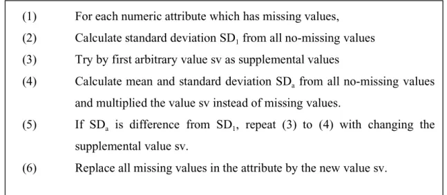
(22) Method Linear regression Standard deviation method Mean and mode Nearest neighbor Autoassociative neural network Decision tree imputation Casewise delation Lazy decision tree Dynamic path generation C4.5 Surrogate split. Reference Pyle, 1999 Pyle, 1999 Han, 2001 Pyle, 1999 Pyle, 1999 Quinlan, 1986 Liu, 1997 Friedman, 1996 White, 1987 Quinlan, 1993 Breiman, 1984. Group Pre-replacing Pre-replacing Pre-replacing Pre-replacing Pre-replacing Pre-replacing Embedded Embedded Embedded Embedded Embedded. Approach Statistic Statistic Statistic Machine learning Machine learning Machine learning Machine learning Machine learning Machine learning Machine learning Machine learning. Table 3-1: Methods for dealing with missing values. 3.2.1 Statistical methods Linear regression: When any two attributes have a correlation, we can make an equation of their relationship and predict the missing values by using the equation if either attribute value is known [Pyle, 1999].. Replacement under same standard deviation: The idea of this method is to fill up missing values by a value that will not disturb each attribute s standard deviation [Pyle, 1999]. See Fig. 3-3.. 14.

(23) (1). For each numeric attribute which has missing values,. (2). Calculate standard deviation SD1 from all no-missing values. (3). Try by first arbitrary value sv as supplemental values. (4). Calculate mean and standard deviation SDa from all no-missing values and multiplied the value sv instead of missing values.. (5). If SDa is difference from SD1, repeat (3) to (4) with changing the supplemental value sv.. (6). Replace all missing values in the attribute by the new value sv. Fig. 3-3: Algorithm for replacement under same standard deviation. Mean and mode method: The idea of this method is using the mean value for numerical attribute and the most frequent value (mode) for symbolical attribute in the whole dataset to fill up missing values [Han, 2001]. See Fig. 3-4.. (1) For each attribute which has missing values, (2) If the attribute is numeric, calculate mean values from all no-missing values. (3) Else, if the attribute is symbolic, count the number of each value and take the value that occurs most frequent. (4) Replace missing values by the computed value.. Fig. 3-4: Algorithm for mean and mode method. 3.2.2 Machine learning methods. 15.

(24) Nearest neighbor estimator: Firstly, this method will find the nearest neighbor instance that includes no missing values for an instance that has missing values. Secondly, it fills up missing values of this instance by the corresponding values of the nearest neighbor instance. To estimate a distance between an instance containing missing values and other instances including no missing values, we can use any available measures Euclidian, Mahalanobis, etc. [Pyle, 1999]. See Fig. 3-5. (1). For each instance Ii which has missing values,. (2). For each instance Ij which has no missing values,. (3). Calculate distance dij between instance Ii and Ij.. (4). Decide the nearest instance In to instance Ii.. (5). Replace each missing value in Ii by the corresponding value in In .. Fig. 3-5: Algorithm for nearest neighbor estimator. Distance estimation To calculate the distance, there are some methods. The Euclidean measure is described by the following equation where m is the number of attribute d ij =. m. ∑(x k =1. ik. − x jk ) 2. Another measure, the Mahalanobis distance [Mahalanobis] is described by the following equation where m is the number of attribute and n is the number of instances. m. m. d ij = ∑∑ ( xil − x jl ) s lk ( xik − x jk ) l =1 k =1. where, slk =. 1 n ∑ ( xil − xl )( xik − xk ) n i =1. 16.

(25) Autoassociative neural networks: This method uses a neural network to deal with missing values. Firstly, the network learns from instances that have no missing values. It is trained to duplicate all of the inputs as outputs by using back propagation. Secondly, when missing values are detected, the network can be used in a back-propagation mode but not a training mode, as no internal weights are adjusted. Instead, the error are propagated all the way back to the inputs. At the input, an appropriate weight can be derived for the missing values so that it least disturbs the internal structure of the network. The values so derived for any set of inputs reflects, and least disturbs, the nonlinear relationship captured by the autoassociative neural network [Pyle, 1999]. See Fig. 3-6. (1). All symbolic attributes are vectorized and all numeric attributes are normalized into [-1,1].. (2). Make a neural network with random weights.. (3). For each no-missing instance,. (4). Learn network that all input values and output values are approximately same by back propagation algorithm.. (5). For each missing instance,. (6). Input values of the instance, where zero values are used for missing values.. (7). If input values and outputs are not same except for the neurons for missing attribute, repeat (6). At that time, the output values are used as input values.. (8). Replace missing values by the output of network.. Fig. 3-6: Algorithm for autoassociative neural network. Decision Tree imputation: This method is to use a decision tree approach to fill up missing values of an attribute. It considers the subset S of the training set S, which consists of instances whose values on an attribute A has no missing values. In S , the original class attribute is regarded as another attribute while the attribute A becomes the class attribute to be determined. Using S , a classification tree can be built for determining values, of attribute A. 17.

(26) from other attributes and the class attribute. Then, this tree can be used to classify each object in the set S-S . Consequently, each missing value can be estimated [Quinlan, 1986]. See Fig. 3-7.. (1) Divide the dataset S into the two subsets Sk and Sm, where Sk consists of instances which have no missing values, Sm consists of instances all of which have missing value(s). (2) For each attribute A in Sk, where A has missing values in Sm, (3). Make decision tree to predict the values of attribute A by all attribute values except for A.. (4) For each instance I in Sm, where I has missing values in Sm. (5). Predict missing values for each corresponding decision tree. Fig. 3-7: Algorithm for decision tree imputation. 3.2.3 Embedded methods Casewise delation: The simplest way to deal with unknown attribute values is just to ignore the instances containing them [Liu, 1997].. Lazy decision tree: Algorithms for constructing decision trees, such as C4.5 [Quinlan, 1993] and CART [Breiman, 1984] create a single best decision tree during the training phase, and this tree is then used to classify test instances. Lazy decision tree conceptually constructs the best decision tree for each test instance. So if a test instance has a missing value, it makes a decision tree with all attributes in the training data set except the attribute on which the test instance has missing values [Friedman, 1996].. Dynamic path generation: Instead of generating the whole decision tree beforehand, this method produces only the path (i.e., the rule) required to classify the instance currently under consideration. Once a missing value is found in an attribute of a new instance, such an. 18.

(27) attribute is never branched on when classifying the instance. In more detail, let us consider the process of building a classification rule (i.e., a path in a classification tree) to classify a new instance O1. At each step, the inductive algorithm chooses the most informative attribute on which to branch. However, if the value of the selected attribute is missing in instance O1, then this attribute cannot be branched on and the algorithm tries with the second most informative attribute. Thus, path generation is strictly dynamic [White, 1987].. C4.5: The system was constructed by Quinlan [1993]. It can not only induce decision trees but also induce rule sets. The rules of decision tree are easy to understand. In this approach, how to deal with missing values in the training phase (making a decision tree) and the testing one (classifying unknown class) are different. On the training phase, if missing values occurred at an attribute that is used for branching, it creates a new branch called unknown . On the testing phase, if a testing instance has missing values, it explores all available branches (below the current node) and decides the class label by the most probabilistic value. This method assumes that unknown test results are distributed probabilistically in proportion to relative frequent of known result.. Surrogate split (CART): When a missing value is found in the attribute originally chosen, the surrogate attribute is the one that has the highest correlation with the original attribute [Breiman, 1984]. 3.3 Evaluation This section gives a brief theoretical evaluation of the above algorithms and an experimental comparative evaluation on several well-known methods to see their effectiveness. In this experiment, we compare five methods on nine data sets. These methods include standard deviation, mean and mode, nearest-neighbor estimator, decision tree imputation and C4.5. Datasets are taken from UCI repository [UCI]. They are the datasets whose attributes are all numerical, all symbolical or mixed. These numbers of instances vary. 19.

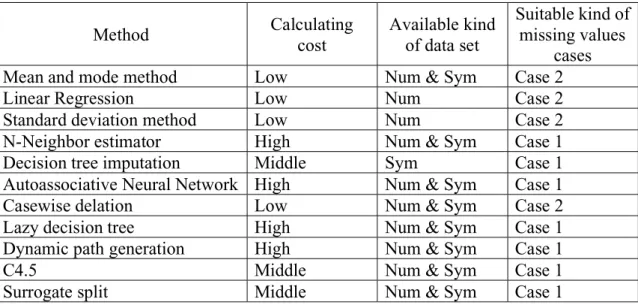
(28) from one hundred to two thousands.. 3.3.1 Theoretical evaluation We tried to analyze methods to deal with missing values in the three following aspects (1) computation cost, (2) available kinds of attributes, (3) suitable cases of missing values. On the first aspect, statistical methods are of low computation cost. Although the decision tree imputation approach is good for generating knowledge from data, it cannot be used for replacing missing values. On the second aspect, three methods can deal with missing values only for one type of attribute, numerical or symbolical. Linear regression and standard deviation methods can work on numeric attribute. Decision tree approach can work on only with symbolic attributes. If required to use these methods, a discretization of numerical attributes is needed. Nearestneighbor method is good at dealing with datasets whose attributes are almost numerical. On the third aspect, statistical methods are suitable when missing values are distributed on some instances (case 1). Others are suitable when missing values are distributed on some attributes (case 2). When the dataset has many missing values, casewise delation leads much bias. See Table 3-2. Standard deviation method seems better than mean method, but it needs to select which value is suitable from two candidate values. Another problem is when a data set is huge, to know the supplemental value is too complicated, especially many values are missing on in one attribute. Nearest neighbor estimator in many cases can be very effective, however, its main drawbacks are that having the training data set available, it may require very big storage. Lookup times for neighbors can be very slow, so finding replacement values is slow, too. In autoassociative neural network, as with any neural network, its internal complexity determines the network s ability to capture nonlinear relationships. Determining that any particular network has, in fact, captured the extant nonlinear relationship is difficult. The. 20.

(29) autoassociative neural network approach has been used with success in replacing missing values for data sets of modest dimensionality (tens and very low hundreds of inputs), but building such networks for moderate- to high-dimensionality data sets is problematic and slow. The amount of data required to build a robust network becomes prohibitive, and for replacement value generation a robust network that actually reflects nonlinearities is needed. At run time, replacement values can be produced fairly quickly. In casewise delation, clearly, when a data set has many instances that have missing values, this method may cause a huge loss of data and, as a result, may not be satisfactory. The effect of surrogate method obviously depends on the magnitude of the correlation in the database between the original attribute and its surrogate.. Method Mean and mode method Linear Regression Standard deviation method N-Neighbor estimator Decision tree imputation Autoassociative Neural Network Casewise delation Lazy decision tree Dynamic path generation C4.5 Surrogate split. Calculating cost Low Low Low High Middle High Low High High Middle Middle. Available kind of data set Num & Sym Num Num Num & Sym Sym Num & Sym Num & Sym Num & Sym Num & Sym Num & Sym Num & Sym. Suitable kind of missing values cases Case 2 Case 2 Case 2 Case 1 Case 1 Case 1 Case 2 Case 1 Case 1 Case 1 Case 1. Table 3-2: Theoretical evaluation of methods for dealing with missing values. 3.3.2 Experimental comparative evaluation 3.3.2.1 Methodology In our experiments the datasets with missing values are obtained in the following way. We start with datasets without missing values. For each of them, we randomly pull out a number of its values in order to make it containing missing values. We pull out only one value on each instance. The rates of values pulled out are 5%, 10% and 20%, respectively. Then, pre-. 21.

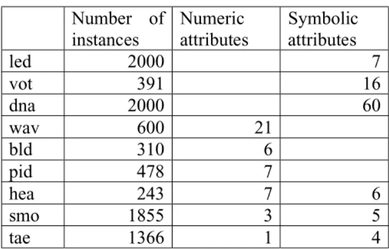
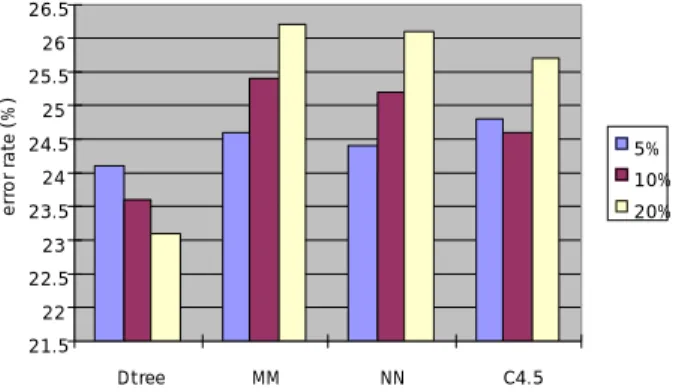
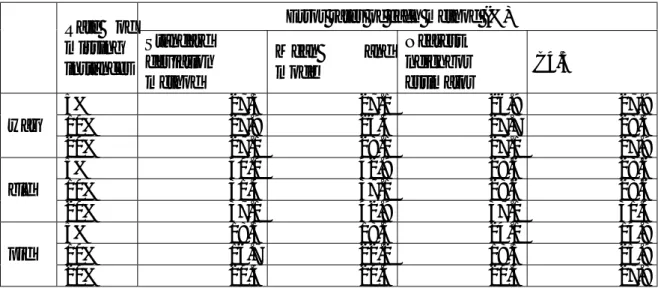
(30) replacing methods are applied to the datasets that include missing values in order to obtain a non-missing value set. Finally, for comparing the effectiveness of the above methods, we apply C4.5 to the obtained non-missing value sets. We used nine datasets, among them the datasets led, vot and dna contain only symbolic attributes; wav, bld and pid contain only numeric attributes; and hea, smo and tae contain both numerical and symbolic attributes. We summarize information of these datasets in Table 3-3.. led vot dna wav bld pid hea smo tae. Number of Numeric Symbolic instances attributes attributes 2000 7 391 16 2000 60 600 21 310 6 478 7 243 7 6 1855 3 5 1366 1 4 Table 3-3: Parameters of data sets. To fill up missing values, we used four methods. Among statistical methods, mean and mode method and standard deviation method are used. Among machine learning methods, nearest neighbor estimator and decision tree imputation methods are used. We apply the embedded method C4.5 to classify non-missing datasets filled up by the four methods, and estimate error rate of these datasets. The last column in each Table 3-4, 3-5 and 3-6 shows error of C4.5 applied to missing value datasets in order to compare the effect of processing missing values directly or indirectly.. 3.3.2.2 Results on datasets with symbolic attributes Three kinds of datasets are compared respectively. The results of each method are summarized Table 3-4, where the smallest errors are in bold.. 22.

(31) Data set. Led. Vot. dna. Error rates of each method (%) Rate of Mean Nearest missing Decision and neighbor C4.5 instances tree imputation mode estimator 5% 24.1 24.6 24.4 24.8 10% 23.6 25.4 25.2 24.6 20% 23.1 26.2 26.1 25.7 5% 0.0 0.0 0.0 0.1 10% 0.0 0.0 0.0 0.1 20% 0.0 0.0 0.1 0.2 5% 1.2 1.2 1.2 1.2 10% 1.2 1.2 1.2 1.2 20% 1.1 1.1 1.2 1.3. Table 3-4: Error rates on the datasets with symbolic attributes. 26.5 26 error rate (% ). 25.5 25 24.5. 5%. 24. 10%. 23.5. 20%. 23 22.5 22 21.5 Dtree. MM. NN. C4.5. Fig. 3-8: Comparing methods by error rates on led data set Decision tree approach achieves lowest error rates of four.. 23.

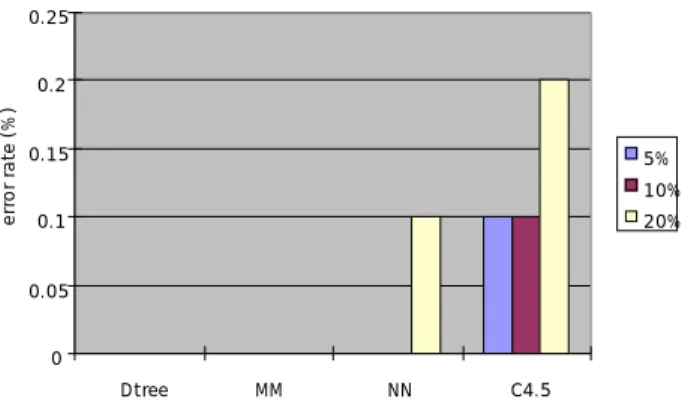
(32) 0.25. error rate (% ). 0.2. 0.15. 5% 10%. 0.1. 20%. 0.05. 0 Dtree. MM. NN. C4.5. Fig. 3-9: Comparing methods by error rates on vot data set Decision tree imputation and mean and mode methods classify perfectly. 1.35. error rate (% ). 1.3 1.25 5%. 1.2. 10% 1.15. 20%. 1.1 1.05 1 Dtree. MM. NN. C4.5. Fig. 3-10: Comparing methods by error rates on dna data set Differences are seen at the rate of 20%. From Fig. 3-8, 3-9 and 3-10, we can observe the followings. On led data set (Fig. 3-8), decision tree imputation is the best one. On vot data set (Fig. 3-9), decision tree imputation and mean and mode methods achieve good results and C4.5 gets the worst one. On dna data set (Fig. 3-10), the one at 20% of instances have a missing value, decision tree imputation and mean and mode achieve good results and C4.5 gets the worst. From these results, we may say that the two methods, decision tree imputation and mean-mode method are good methods to deal with missing values when attributes are all symbolic.. 3.3.2.3 Results on datasets with numeric attributes. 24.

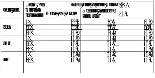
(33) pid. 27.3 27.9 27.1 40.0 31.4 37.1 18.5 16.7 20.4. Error rates of each method (%) Nearest Mean and neighbor C4.5 mode estimator 27.1 26.9 26.4 27.7 28.1 27.1 42.9 28.6 37.1 28.6 42.9 37.1 18.5 24.1 22.2 18.5 20.4 20.4. Table 3-5: Error rates on the datasets with numeric attributes. 29 28.5 28 error rate (% ). bld. 27.5. 5%. 27. 10% 20%. 26.5 26 25.5 25 SD. MM. NN. C4.5. Fig. 3-11: Comparing methods by error rates on wav data set It seems that nearest neighbor estimator achieves low error rates. 50 45 40 error rate (% ). wav. Rate of missing Standard instances deviation method 5% 10% 20% 5% 10% 20% 5% 10% 20%. 35 30. 5%. 25. 10%. 20. 20%. 15 10 5 0 SD. MM. NN. 25. C4.5. 27.9 28.5 27.9 28.6 28.6 31.4 14.8 25.9 27.8.

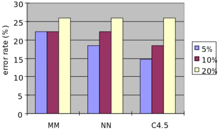
(34) Fig. 3-12: Comparing methods by error rates on bld data set Nearest neighbor and C4.5 achieve lower error rate than other two. 30. error rate (% ). 25 20 5% 15. 10% 20%. 10 5 0 SD. MM. NN. C4.5. Fig. 3-13: Comparing methods by error rates on pid data set Standard deviation method seems the best one. Fig. 3-11, 3-12 and 3-13 show graph of Table 3-5. On wav data set (Fig. 3-11), although there is some different tendency depending on the rate of missing values, nearest neighbor estimator obtained the best result of the four methods. On bld data set (Fig. 3-12), the nearest neighbor estimator and C4.5 are the best ones. On pid data set (Fig. 3-13), standard deviation method achieves better result than others. From the whole error rates, we may say that standard deviation method and nearest neighbor estimator are preferred for dealing with missing values on numeric attributes.. 3.2.2.4 Results on datasets with mixed attribute. Data set. hea. smo. tae. Error rates of each method (%) Ratio of missing Nearest neighbor C4.5 instances Mean and mode estimator 5% 22.2 18.5 10% 22.2 22.2 20% 25.9 25.9 5% 34.9 34.9 10% 35.4 36.2 20% 34.6 34.3 5% 46.7 46.7 10% 46.7 53.3. 26. 14.8 18.5 25.9 34.9 35.5 34.7 46.7 53.3.

(35) 20%. 53.3. 53.3. 53.3. Table 3-6. Error rates on the datasets with mixed attributes. error rate (% ). 30 25 20 5% 10% 20%. 15 10 5 0 MM. NN. C4.5. Fig. 3-14: Comparing methods by error rates on hea data set The error rates of C4.5 are lowest of all three methods. 36.5. error rate (% ). 36 35.5 5%. 35. 10% 34.5. 20%. 34 33.5 33 MM. NN. C4.5. Fig. 3-15: Comparing methods by error rates on smo data set Differences are seen at the rates of 10% and 20%.. 27.

(36) 54. error rate (% ). 52 50 5% 10%. 48. 20% 46 44 42 MM. NN. C4.5. Fig. 3-16: Comparing methods by error rates on tae data set Ncbmm is lowest at the rate of 10%. Fig. 3-14, 3-15 and 3-16 are graph of Table 3-6. On hea data set (Fig. 3-14), C4.5 is the best one. On smo (Fig. 3-15) and tae data sets (Fig. 3-16) mean and mode method has the lowest error rates than others. The whole results on these three subsections show that; ・ decision tree estimator and mean-mode method are good methods for dealing with missing values on symbolic attributes, ・ nearest neighbor method and standard deviation method are good methods for dealing with missing values on numeric attributes, ・ mean and mode method gives good results generally. One simple method, mean and mode method, can give results as good as other complicated methods. Especially for the datasets which attributes are mixed, it may be a good method.. 28.

(37) Chapter 4. 4.1 Basic idea of scalable algorithms For large data sets with missing values, complicated methods are not suitable because their computation costs prevent them from computing on large datasets. We tend to find simple methods that can reach performance as high as complicated ones. The results and experience obtained in the previous chapter suggested us to come to simple but efficient solution to fill up missing values in large datasets. According to the result of the last experiments, mean and mode method showed as good results as C4.5. We may say that mean and mode method can have high performance to missing values problem for large datasets, and can be efficient and scalable for large data sets with necessary improvements. Our approach to this problem is based on variants of mean and mode method and k-means. The basic idea of our method is the cluster-based filling up of missing values. Instead of using. 29.

(38) mean and mode on the whole dataset we use mean and mode in its subsets obtained by clustering. It consists of three variants of the mean and mode algorithm: 1. Natural Cluster Based Mean and Mode algorithm (NCBMM), 2. attribute Rank Cluster Based Mean and Mode algorithm (RCBMM), 3. k-Means Clustering Based Mean and Mode algorithm (KMCMM). NCBMM uses the class attribute to divide instances in to natural classes and uses the mean of each natural cluster to fill up missing values on numeric attributes of instances belong to the cluster, and mode of natural clusters to fill in the missing values of cluster instances for symbolic attributes. This algorithm is the simplest improvement of mean and mode algorithm in case of supervised data but as shown in next sections it is very efficient if applicable. RCBMM and KMCMM divide dataset into subsets by using the relationship between attributes. The starting point of these algorithms came from the question, Is the class attribute always the key attribute for clustering an arbitrary descriptive attribute? For some attributes, some of descriptive attributes may be better for clustering than the lass attribute. The remark that to cluster instances concerning one missing attribute, the key attribute selected from all attributes may give better results than NCBMM. It is also an available solution for unsupervised data. We describe these algorithms in next section.. 4.2 The proposed algorithms NCBMM algorithm can be applied to supervised data where missing value attributes can be either symbolic or numeric. It produces a number of subsets equal the number of class values. At first, the whole instances are divided into clusters, where instances of each cluster have the same values of the class attribute. Then, in each cluster, the mean value is used to fill up missing values for each numeric attribute, and the mode value is used to fill up missing values for each symbolic attribute. We describe the algorithm in Fig. 4-1.. 30.

(39) (1) Divide all instances into clusters by the class label (2) For each cluster, (3) (4). For each attribute which has missing values, For a numeric attribute, calculate mean values from all no-missing Values.. (5). For a symbolic attribute, find the most probable value.. (6). Fill up missing values by the mean or mode value. Fig. 4-1: Algorithm NCBMM. RCBMM can be applied to filling up missing values for symbolic attributes independently with the class attribute. Therefore, it can be applied to both supervised and unsupervised data. Firstly, for one missing attribute, this method ranks attributes by their distance to the missing value attribute. The attribute that has smallest distance is used for clustering. Secondly, all instances are divided into clusters each contains instances having the same value of the nearest attribute. Thirdly, the mode of each cluster is used to fill up missing values. This process is applied to each missing attribute. We describe the algorithm in Fig. 4-2.. (1) For each missing attribute ai (2). Make a ranking of all n symbolic attributes in decreasing order of distance between ai and each attribute aj. (j ∈ 1. (3). n, j ≠ i). Divide all instances into clusters based on the values of ah, where ah is The attribute, which has the highest rank from attribute ai.. (4). Replace missing value on attribute ai by the mode of each cluster.. (5). Repeat from 2 to 4 till all missing values on attribute ai are replaced where h changes to the next number of ranking.. Fig. 4-2: Algorithm RCBMM. 31.

(40) We can use several measures to calculate distance between attributes. Our idea is to measure how two attributes have similar distributions of values. Quinlan used information gain in order to know that in C4.5 [1993]. A disadvantage of this measure is that it is biased towards selecting attributes with many values. Mantaras [1991] proposed the new measure to calculate distance between partitions of two attributes to solve this problem. It is defined as following, where PA and PB denote two values partition of attributes A and B.. d N ( PA , PB ) =. d ( PA , PB ) I ( PA ∩ PB ). where Pi = P( Ai ) Pj = P( B j ) Pij = P( Ai ∩ B j ) Pj / i = P( B j / Ai ). For all 1 ≤ i ≤ n and 1 ≤ j ≤ m n. I ( PA ) = − ∑ Pi log 2 Pi i =1 m. I ( PB ) = − ∑ Pj log 2 Pj j =1. n. m. I ( PA ∩ PB ) = − ∑∑ Pij log 2 Pij i =1 j =1. n m n m  Pij  I ( PB / PA ) = I ( PB ∩ PA ) − I ( PA ) = − ∑ ∑ P ij log 2   = − ∑ Pi ∑ Pj / i log 2 Pj / i i =1 j =1 i =1 J −1  Pi  d ( PA , PB ) = I ( PB / PA ) + I ( PA / PB ). KMCMM can be applied to filling up missing values for symbolic attributes. 32.

(41) independently with the class attribute. Therefore, it can be applied to both supervised and unsupervised data. K-means algorithm is used for ranking numerical attributes. We describe the algorithm for KMCMM in Fig. 4-3.. (1) For each missing attribute ai (2). Make a ranking of all n numeric attributes in increasing order of absolute values of correlation coefficient between attribute ai and each attribute aj. (j ∈ 1. (3). n, j ≠ i). Divide all instances by k-mean algorithm based on the values of ah, where ah is the attribute that has the highest rank from attribute ai.. (4). Replace missing value on attribute ai by the mode of each cluster.. (5). Repeat from 2 to 4 till all missing values on attribute ai are replaced where h Fig. 4-3: Algorithm KMCMM. Correlation Coefficient The value of r is calculated from n pairs of observations (x, y) according to the following formula: r=. S xy S xx S yy. where S xy = ∑ ( x − x )( y − y ) S xx = ∑ ( x − x )2. S yy = ∑ ( y − y )2. 33.

(42) k-Means Clustering Algorithm The k-means algorithm proceeds as follows. First, it randomly selects k of the objects, each of which initially represents a cluster mean or center. For each of the remaining objects, an object is assigned to the cluster to which it is the most similar, based on the distance between the object and the cluster mean. It then computes the new mean for each cluster. This process iterates until the criterion function converges. Typically, the squared-error criterion is used, defined as E = ∑i =1 ∑ p∈C | p − mi |2 , k. i. where E is the sum of square-error for all objects in the database, p (pls change this notation) is the point in space representing a given object, and mi is the mean of cluster Ci (both p and mi are multidimensional). This criterion tries to make the resulting k clusters as compact and as separate as possible. The k-means procedure is summarized in fig. 4-4.. (1). Arbitrarily choose k objects as the initial cluster centers;. (2). Repeat. (3). (re)assign each object to the cluster to which the object is the most similar, based on the mean value of the objects in the cluster;. (4). Update the cluster means, i.e., calculate the mean value of the objects for each cluster;. (5). Until no change; Fig. 4-4: Algorithm for k-means clustering. 4.3 Evaluation 4.3.1 Methodology To evaluate the performance of pre-replacing methods our method consists of two phases:. 34.

(43) (1) filling up missing values on data set by replacing methods and measure the executing time, (2) evaluating the quality of the replaced datasets by different in terms of error rate in classification. In other words, firstly each non-missing value dataset is obtained from the dataset that has missing values by replacing methods to be evaluated. Secondly, we apply the same data mining methods (C4.5 in our study) to non-missing value datasets obtained by different replacing methods and comparing their quality of these datasets (i.e. the quality of replacing methods). Six replacing methods, NCBMM, RCBMM, KMCMM, nearest neighbor estimator, autoassociative neural network and decision tree imputation and one embedded method, C4.5, are used for this comparative evaluation. For evaluating the quality of replaced datasets, three classification methods, C4.5, Na ve Bayesian classifier, k-nearest neighbor classifiers are used. Fifteen data sets were replaced and classified. They are from UCI repository [UCI]. There are three types of datasets: all attributes are numerical (except for class attribute), symbolic and mixture of symbolic and numeric. They have missing values originally. The parameters of each data set are summarized in Table 4-1, 4-2 and 4-3, where the column of Num , Sym mean the number of attribute for numeric, symbolic respectively. Numerator values are the number of attributes that has missing values, and denominator value is the number of attributes. Num Sym Class Missing values cases cmc 2/2 1/7 3 Case 1 edu 8/8 2/4 4 Case 1 and 2 hco 5/5 13/14 2 Case 2 lbw 1/2 2/6 2 Case 1 smo 1/3 1/5 3 Case 1. Missing instances / all instances 2002/14730 (13.6%) 9990/10000 (99.9%) 3290/3680 (89.4%) 240/1890 (12.7%) 5340/28550 (18.7%). Table 4-1: Data sets those have missing values on both numeric and symbolic attributes. NumSym Class Missing values cases hab 3/3 2 Case 3 sat 2/36 6 Case 1 wav 3/21 3 Case 1. 35. Missing instances / all instances 562/3060 (18.4%) 1195/6435 (18.6%) 674/3600 (18.7%).

(44) Table 4-2: Data sets those have missing values on numeric attributes. NumSymClass Missing values cases adt 0/6 2/7 2 Case 1 and 2 att 0/1 8/8 2 Case 1 and 2 dna 3/60 3 Case 1 hin 5/6 3 Case 1 inf 2/18 6 Case 1 led 7/7 10 Case 3 tae 1/1 4/4 3 Case 3. Missing instances / all instances 1335/22747 (5.9%) 2430/10000 (24.3%) 354/2372 (14.9%) 4050/10000 (40.5%) 250/2380 (10.5%) 1770/6000 (29.5%) 120/1510 (7.9%). Table 4-3: Data sets those have missing values on symbolic attributes.. 4.3.2 Analysis of results We tried to compare methods for dealing with missing values, by error rates of three classifiers C4.5, Na ve Bayesian classifier and k-nearest neighbor classifier after replacing and counting execution time of replacing.. 4.3.2.1 Error rate In this subsection we first report the results of experience with C4.5 classification program, Na ve Bayes classification, and k-nearest neighbor classification. We then summarize theses results in two tables that show the order or methods for filling up missing values in terms of three classification methods.. 36.

(45) With C4.5 classifier NCBMM RCBMM KMCMM 5.2 5.5 5.5 0.0 0.0 0.0 0.0 0.0 0.0 3.9 3.9 3.9 1.3 1.3 1.3. NN. annet 4.7 1.8. 5.2 1.9. 4.7 1.6. Table 4-4: Error rates on mixed data sets (%). 8 7 6 error rate (% ). cmc edu hco lbw smo. C4.5 6.7 5.2 0.9 5.1 2.2. C4.5 NCBMM RCBMM KMCMM NN annet. 5 4 3 2 1 0 cmc. edu. hco. lbw. smo. Fig. 4-5: Error rates of each method on mixed data set Three clustering methods achieved low error rate generally.. 37. DT.

(46) C4.5 4.3 13.1 24.5. NCBMM RCBMM KMCMM 2.9 2.9 13.6 14.1 24.0 23.5. NN 13.5 24.6. annet 3.8 13.1 24.4. Table 4-5: Error rates on numeric data sets (%). 30. 25. error rate (% ). hab sat wav. 20 C4.5 NCBMM KMCMM NN annet. 15. 10. 5. 0 hab. sat. wav. Fig. 4-6: Error rates of each method on numeric data set There is a not so big difference here.. 38. DT.

(47) Adt Att Dna Hin Inf Led Tae. C4.5 15.1 2.2 4.7 12.9 2.4 29.1 2.8. NCBMM RCBMM KMCMM 15.2 15.1 1.2 1.2 4.7 4.7 9.0 10.6 2.3 2.3 25.1 25.1 2.8 4.0. NN. annet Nan 1.1 11.3 2.4 32.0. DT 15.2 2.3 4.6 10.4 2.4 25.2. Table 4-6. Error rates on symbolic data sets (%). 35. error rate (% ). 30 25 C4.5 NCBMM RCBMM annet DT. 20 15 10 5 0 adt. att. dna. hin. inf. led. tae. Fig. 4-7: Error rates of each method on symbolic data sets There are somehow different error rates on hin and led data set. C4.5 and autoassociative neural network achieve higher error rates than others.. With Na ve Bayesian classifier. 39.

(48) NCBMM RCBMM KMCMM 49.5 50.5 49.5 18.1 18.2 41.5 10.9 16.0 10.9 28.6 28.6 28.6 31.7 31.7 31.7. cmc edu hco lbw smo. NN. annet 51.4 45.5. 28.4 31.1. 27.4 31.0. DT. Table 4-7: Error rates on mixed data sets (%). 60. error rate (% ). 50. 40 NCBMM RCBMM KMCMM NN annet. 30. 20. 10. 0 cmc. edu. hco. lbw. smo. Fig. 4-8: Error rates of each method on mixed data set On edu data set, KMCMM and autoassociative neural network achieve worse results than others. On hco data set, RCBMM is the worst one among three. NCBMM is stably good.. hab sat wav. NCBMM RCBMM KMCMM 24.6 24.6 23.6 24.3 14.9 15.7. 40. NN 24.3 15.9. annet 24.6 24.1 15.7. DT.

(49) Table 4-8: Error rates on numeric data sets (%). 30. error rate (% ). 25. 20 NCBMM KMCMM NN annet. 15. 10. 5. 0 hab. sat. wav. Fig. 4-9: Error rate of each method on numeric data sets There is not much difference. Nearest neighbor estimator can t deal with hab data set because there is not any attribute that has no missing values.. adt att dna hin inf led tae. NCBMM RCBMM KMCMM 18.2 18.2 36.0 36.7 4.2 4.2 20.4 23.3 20.0 20.0 25.2 25.2 33.7 37.7. 41. NN. annet 38.7 26.3 21.3 31.1. DT 18.3 36.2 4.6 24.1 20.1 25.1.

(50) Table 4-9: Error rates on symbolic data sets (%). 45 40. error rate (% ). 35 30 NCBMM RCBMM annet DT. 25 20 15 10 5 0 adt. att. dna. hin. inf. led. tae. Fig. 4-10: Error rates of each method on symbolic data sets Autoassociative neural network is the worst one among four methods. On adt data set, autoassociative neural network can t work because the number of neurons is too big.. With k-nearest neighbor classifier. cmc edu hco lbw smo. NCBMM RCBMM KMCMM 4.6 4.8 4.6 0.0 0.0 0.0 0.0 0.0 0.0 3.5 3.5 3.5 1.1 1.1 1.1. NN. annet 3.9 1.9. 4.7 1.8. 4.1 1.4. Table 4-10: Error rates on mixed data sets (%). 42. DT.

(51) 6. error rate (% ). 5. 4 NCBMM RCBMM KMCMM NN annet. 3. 2. 1. 0 cmc. edu. hco. lbw. smo. Fig. 4-11: Error rates of each method on mixed data sets On the edu, hco, lbw and smo datasets, three clustering methods are relatively good.. hab sat wav. NCBMM RCBMM KMCMM 2.7 2.7 11.6 11.5 14.4 15.4. NN 11.4 15.5. annet 3.3 12.6 16.1. Table 4-11: Error rates on numeric data sets (%). 43. DT.

(52) 18 16. error rate (% ). 14 12 NCBMM KMCMM NN annet. 10 8 6 4 2 0 hab. sat. wav. Fig. 4-12: Error rates of each method on numeric data sets The error rates are almost same, but autoassociative neural network achieves the highest rate.. adt att dna hin inf led tae. NCBMM RCBMM KMCMM 18.4 18.7 1.3 1.1 9.1 9.1 7.9 10.1 2.4 2.4 25.8 25.8 2.9 3.8. NN. annet 1.0 10.9 2.4 32.5. Table 4-12: Error rates on symbolic data sets (%). 44. DT 18.9 2.0 10.4 2.4 26.1.

(53) 35. error rate (% ). 30 25 NCBMM RCBMM annet DT. 20 15 10 5 0 adt. att. dna. hin. inf. led. tae. Fig. 4-13: Error rates of each method on symbolic data set The error rates are almost same, but autoassociative neural network achieves the highest rate.. From these results, we tried to evaluate the methods. Regarding the accuracy, we describe the order of appropriateness of methods for each numeric and symbolic attribute. We summarize them into Table 4-13 and 4-14 for attribute type, numerical or symbolical. Classifier C4.5 Na ve bayes k-NN. 1st NCBMM C4.5 NCBMM. 2nd KMCMM NCBMM KMCMM. 3rd C4.5 KMCMM NN. 4th annet annet annet. 5th NN NN C4.5. Table 4-13: The order of appropriateness of methods for dealing with missing values on numeric attributes. Classifier C4.5. 1st NCBMM. 2nd RCBMM. 3rd DT. 45. 4th annet. 5th C4.5.

(54) Na ve bayes k-NN. C4.5 NCBMM. NCBMM RCBMM. RCBMM C4.5. DT DT. annet annet. Table 4-14: The order of appropriateness of methods for dealing with missing values on symbolic attributes. These results show that, our clustering methods, NCBMM, RCBMM and KMCMM to replace missing values can be seen as better than considering machine learning methods, autoassociative neural network and nearest neighbor estimator.. 4.3.2.2 Execute time for replacing. cmc edu hco lbw smo. NCBMM RCBMM KMCMM 0:02 0:03 0:02 0:02 0:02 0:04 0:01 0:03 0:05 0:00 0:00 0:00 0:03 0:03 0:03. NN. annet 92:29 0:25. 0:01 4:26. 1:16 28:52. DT. Table 4-15: Execute time for replacing on mixed data sets (min: sec). hab sat wav. NCBMM RCBMM KMCMM 0:00 0:00 0:03 0:11 0:01 0:05. NN 3:46 0:39. annet 0:02 54:03 26:19. DT. Table 4-16: Execute time for replacing on numeric data sets (min: sec). adt att. NCBMM RCBMM KMCMM 0:03 0:06 0:04 0:03. 46. NN. annet. DT 37:49 2:09.

(55) dna hin inf led tae. 0:01 0:01 0:01 0:01 0:00. 0:01 0:02 0:01 0:01 0:00. 124:13 212:10 113:00. 0:03 0:04 0:01 0:06. Table 4-17: Execute time for replacing on symbolic data sets (min: sec). Table 4-15, 4-16 and 4-17 show us that NCBMM, RCBMM and KMCMM are much faster than other methods.. 4.3.3 Experiment on census-income data set We tried to compare the methods for a huge data set. Here, we used census-income dataset. It has 299,285 instances and in this dataset there are 156,764 missing instances. They are more than half of the dataset. This set has eight numeric and thirty-three symbolic attributes except the class attribute. Each value on the class attribute can take one of two labels. Missing values exist on only symbolical attributes. See5 is used for classifying. It is the latest version of C4.5. We compared the error rate of See5 obtained directly, and that of See5 obtained after replacing missing values by NCBMM and RCBMM. And we measured the execution time for preparing at each replacing method. Here, we used Ultra spark machine and Sun-UNIX as operating system for this computing. See Table 4-18.. See5 NCBMM RCBMM. Error rate (%) 4.6 4.6 4.6. Time for preparing (sec.) N/A 171.41 651.38. Table 4-18. Comparing replaced methods and direct processing method. Error rates of all replaced datasets are same. And the computation time shows that NCBMM and RCBMM methods are scalable.. 47.

(56) Chapter 5 Conclusion and future work. 5.1 Comparing the methods Firstly, we compared theoretically several well-known existing methods to deal with missing values in chapter 3. Some of them can be applied to either numeric or symbolic attributes. And, it turns out that the processing cost of missing values is different greatly in different methods. Secondly, we compared experimentally them. Some methods can impute missing values with high accuracy. Nearest neighbor estimator and decision tree imputation sometimes showed good results. However, in terms of synthetic view and computation cost, it can be said that the result with mean and mode method is sufficient good. This was as good as the result of C4.5 that is one of typical classifiers which processed missing values directly. The most important problem in this field is how to reduce processing cost because the data to process is larger day by day in the actual world. Fortunately, it showed that our methods based on clustering could deal with missing values as good as other complicated methods and with low cost. Thus, it is shown that they can be applied to large datasets.. 48.

(57) 5.2 Scalable algorithms to deal with missing values NCBMM, RCBMM and KMCMM, our proposed algorithms for dealing with missing values can replace missing values as good as other complicated methods. The advantages of our methods are the followings.. ・ They are not specialized for one data mining method. In other words, they are not built in methods for dealing with missing values. They offer a high applicability to KDD when most datasets have missing values. ・ They can deal with missing values with low cost and as accurate as other methods. It shows that they can deal with huge datasets that have missing values. ・ RCBMM and KMCMM can be applied to unsupervised datasets, because they do not need to use the class attribute.. We did an experiment to evaluate NCBMM and RCBMM in a large data set that consists missing values in chapter 4. By the result, they achieved as same accuracy as the result of classifying by See5. Moreover, they took for processing about 3 and 11 minutes respectively. It can be said that these are scalable to large datasets.. 5.3 Future work As a future subject,. 49.

(58) ・ Though the obtained results are interesting and very encouraging, it could be considered as an initial work in this research direction for dealing with missing values. This research is hopefully to be pursued, refined and verified with a large number of datasets, and with other alternative methods of evaluation. ・ We must check effective methods for each missing values cases. Although we experimented in chapter 4 about datasets which has missing values beforehand, we can conduct this experiment using datasets without missing values by removing values for each missing values pattern proposed by chapter 3. If an effective method is known for each missing values case, it will enable data mining software to choose and perform how to replace missing values automatically on the basis of the state of missing values contained in dataset. ・ We must take into consideration the reason for causing of missing values. We are described in chapter 2 that there were two reasons about the cause of missing values. One is on the phase of data collection, when operator judges that the value is to be treated as missing value. Another is the case when a certain value has fallen out by chance by a certain cause on KDD process. These things did not take into consideration by this research. It is thought that this was violent approach. It is also thought that the cause of missing values affects the performance of a method that process missing values. More precious investigation about these influences should be done. ・ We should investigate the validity of RCBMM and KMCMM in detail. Although RCBMM and KMCMM improved NCBMM, this experiment showed the result with the more sufficient NCBMM. As compared with NCBMM, we should investigate about the validity of RCBMM and KMCMM. Moreover, these will be able to be unified, if there is the method of measuring the relevance of numeric and symbolic attribute, although RCBMM was effective in symbolic and KMCMM was effective in numeric attribute.. 50.

(59) Acknowledgement Firstly, I would like to express my profound appreciate to professor Ho Tu Bao for his allround support during the research. He has given me not only appropriate instructions and suggestions but also his warm encouragement, while he has been very busy. I also thank to associate professor Masato Ishizaki for his support in many aspects, professor Akito Sakurai for his suggestions to write a paper of my sub research theme. And professor Setsuo Osuga, in the department of science and engineering in Waseda University gave me significant remarks about experimental methods. Another thanks are to many people who in the knowledge creation methodology seminar, and the school of knowledge science in JAIST, I received many advise, indication, and the inspiration about implementation and research. I appreciate deeply to them. Finally, I express gratitude hearty once again to the above people and all people supported me on my research and my student life until now. February 13, 2001 Yoshikazu Fujikawa. 本研究をすすめるにあたり、Ho Tu Bao 教授には多忙な中にも関わらず、多くの指導、激励、方向性に関する示唆、また英文での論文執筆に関する添削など、様々な面で支えていただきました。石崎雅人助教授には研究のみならず様々な面で応援をしていただきました。櫻井彰人教授には副テーマの論文執筆に多くの助言をいた. 51.

(60) だきました。また実験を進めるに際して、早稲田大学理工学部教授、大須賀節雄先生に示唆を与えていただきました。知識創造論講座の方々や、知識科学研究科の多くの方々に実装や研究に関するアドバイス、ご指摘、アイデアを頂きました。以上の方々と、これまでの私の研究生活・学生生活を支えてくださった全ての方々に厚く御礼申し上げます。ありがとうございました。 2001 年 2 月 13 日冨士川義和. References [Breiman, 1984] Breiman, L., Friedman, J.H., Olshen, R.A. & Stone, C.J.: Classification and regression trees. Belmont: Wadsworth, 1984.. [Friedman, 1996] Friedman, J. H., Khavi, R. & Yun, Y.: Lazy Decision Trees. In proceedings of the 13th National Conference on Artificial Intelligence, pp. 717-724, AAAI Pres/MIT Press, 1996.. [Han, 2001] Han, J. & Kamber, M.: Data Mining: Concepts and Techniques, Morgan Kaufmann Publishers, 2001.. [Kononenko, 1984] Kononenko, I., Bratko, I. & Roskar, E.: Experiments in automatic learning of medical diagnostic rules. Technical Report. Jozef Stefan Institute, Ljubjana, Yugoslavia, 1984.. [Lee, 2000] Lee, K.C., Park, J.S., Kim, Y.S. and Byun, Y.T.: Missing Value Estimation Based on Dynamic Attribute Selection. In proceedings of the PAKDD 2000, pp. 134-137, 2000.. 52.

(61) [Little, 1987] Little, R. J. A. & Rubin, D. B.: Statistical analysis with missing data. 1987, John Wiley & Sons, Inc, 1987.. [Liu, 1997] Liu, W.Z., White, A.P., and Thompson S.G. & BRAMER M.A.: Techniques for Dealing with Missing Values in Classification. In IDA 97, Vol.1280 of Lecture notes, 527-536, 1997. [Lobo, 2000] Lobo, O.O. & Numao, M.: Ordered Estimation of Missing Values for Propositional Learning. 人工知能学会誌 15 巻 1 号, 2000.. [Mannila, 1996] Mannila, H.: Data mining: machine learning, statistics, and databases. Eight International Conference on Scientific and Statistical Database Management, Stockholm June 18-20, 1996, p. 1-8, 1996.. [Mantaras, 1991] Mantaras, R. L.: A Distance-Based Attribute Selection Measure for Decision Tree Induction. Machine Learning, 6, 81-92, 1991.. [Pyle, 1999] Pyle, D.: Data Preparation for Data Mining. Morgan Kaufmann Publishers, Inc, 1999.. [Quinlan, 1986] Quinlan, J.R.: Induction of decision trees. Machine Learning, 1, 81-106, 1986.. [Quinlan, 1993] Quinlan, J. R.: C4.5: Programs for Machine Learning. Morgan Kaufmann Publishers, Inc, 1993.. [UCI] UCI machine learning repository, http://www.ics.uci.edu/~mlearn/MLRepository.html. [Weiss, 1998] Weiss, S. M. and Indurkhya N.: Predictive Data Mining A Practical Guide. Morgan Kaufmann Publishers, Inc, 1998.. 53.

(62) [White, 1987] White, A.P.: Probabilistic induction by dynamic path generation in virtual trees. In Research and Development in Expert Systems III, edited by M.A. Bramer, pp. 35-46. Cambridge: Cambridge University Press, 1987.. 54.

(63)