RIMS-1648
Randomized Approximation for Generalized Median Stable Matching
By
Shuji KIJIMA and Toshio NEMOTO
November 2008
R ESEARCH I NSTITUTE FOR M ATHEMATICAL S CIENCES
KYOTO UNIVERSITY, Kyoto, Japan
Randomized Approximation for Generalized Median Stable Matching
Shuji Kijima∗ Toshio Nemoto† November 11, 2008
Abstract
This paper deals with finding ageneralized median stable matching(GMSM), introduced by Teo and Sethuraman (1998) as a fair stable marriage. Cheng (2008) showed that finding thei-th GMSM is #P-hard in case ofi= O(N), whereN is the number of stable matchings of an instance. She also gave an exact algorithm running in polynomial time in case of i= O(log logN), and the complexity remained as open in case ofiisω(log logN) and o(N).
In this paper, we establish two hardness results. We show that finding thei-th GMSM is #P-hard even wheni= O(N1/c), wherec≥1 is an arbitrary constant, and that deciding if a matching can be a GMSM is #P-hard. On the other hand, we give a polynomial time exact algorithm in case thatiis O((logN)c′) wherec′ is an arbitrary positive constant. We also propose tworandomized approximation schemesfor thei-th GMSM using an oracle for almost uniformly sampling ideals of a partially ordered set (poset). This is the first result on randomized approximation schemes for the GMSM.
Key words: stable marriage, distributive lattice, order ideals, antichains, partially ordered set, #P-hard, FPRAS.
1 Introduction
In thestable marriage problem, sets M of n-men andW of n-women, and lists of each person’s preference over opposite sex are given as an input instance. A matching is n pairs of a man and a woman, in which every person appears exactly once. In a matching, a pair m ∈M and w∈W is calledblocking pair ifm andwprefer each other to each current partner. A matching isstable unless a blocking pair exists.
Gale and Shaplay [6] showed that every instance of the stable marriage problem has a stable matching, and they also gave a finding algorithm. For an instance of the stable marriage problem, some stable matchings exist in general. Conway pointed out the set of all stable matchings for an instance forms a distributive lattice [13]. Furthermore, Blair [2] showed that every distributive lattice can be represented by an instance of the stable marriage problem.
Conway’s note indicates another interesting property of the stable marriage, so-called the
“median property” (see e.g. [23, 8, 13]). Generalizing the property, Teo and Sethuraman [23]
devised an idea of the generalized median stable matching (GMSM), as a fair stable marriage.
Here we briefly explain the GMSM.
Let M be a set of all stable matchings for an instance. Letµi (1≤i≤N) be a matching of M where N def.= |M|, and then µi(m) ∈ W denotes a partner of m ∈ M on the matching
∗Research Institute for Mathematical Sciences, Kyoto University, Japan[email protected]
†Graduate School of Information and Communication, Bunkyo University, Japan
w1
w5 w2 w3 w4
w2 w1 w3
w4 m4
w4
w2
w3
w5
m5
w1 w5 w4
w3 m3
w5 w4 w1
w2 m2
w5 w3 w2
w1 m1
5 5 3 5 3 3 4 4 m4
3 4 1 2 µ7
3 2 1 4 µ8
5 3 1 2 µ2
5 4 2 1 µ3
5 4 1 2 µ4
2 4 3
m3
5 3 5
m5
1 2 2
m2
4 1 1
m1
µ6
µ5
µ1
3 3 3 5 5 5 5 5 m5
5 5 5 3 3 3 4 4 m4
α7
2 1 4
α8
2 1 4
α2
3 2 1
α3
4 2 1
α4
4 1 2
4 4 3
m3
α6
α5
α1
1 1 2
m2
2 2 1
m1 m5
m3 m4 m1 m1
m2 m5 m4 m1
w4
m3
m2
m1
m4
w5
m1 m2 m3 m5
w3
m5 m4 m2 m3
w2
m5 m4 m3 m2
w1
µ1 µ3 µ4 µ7 µ8
Men’s list Women’s list
arrange each row
b. Stable matchings c. GMSMs
a. Preference list
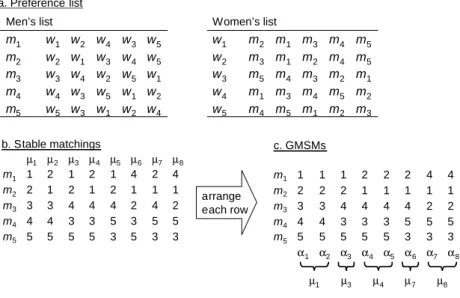
Figure 1: An example of GMSMs.
µi. Now we define M(m) for m ∈ M as the multiset of all µi(m) (1 ≤ i ≤ N). Let α(m) = (α1(m), α2(m), . . . , αN(m)) for m∈M be an arrangement of M(m), in which eachα(m) is in order of preference of each m; i.e., αi(m)∈W is preferable for m or identical to αi+1(m)∈W for all i(1≤i < N). Note that α(m) is independently arranged for m∈M of each other. Let αi (1≤i≤N) be a set ofnpairs ofm∈M andαi(m)∈W, everyαi is again a stable matching inM, that is shown by Teo and Sethuraman [23] using linear programming. We call αi thei-th generalized median stable matching (ori-th GMSM, for short).
Figure 1 shows an example with five men and five women. Figure 1-a shows their preference lists; in Men’s lists, women are arranged in order of each mi’s preference from left to right in each row mi ∈ M, and men are arranged in order of each wi’s preference in Women’s lists.
Figure 1-b shows all stable matchings µ1, . . . , µ8 of the instance. In the table, the number k denotes the index of a womanwk where wk =µj(mi) in the i-th row of the j-th column. Thus each column j ∈ {1, . . . ,8} corresponds to a stable matchingµj. In Figure 1-c, all partners of mi in 8-stable matchings are arranged in the i-th row, according to the preference of each mi; i.e., the i-th row representsα(mi) (with indices k of womenwk =αj(mi)). Then each column α1, . . . , α8 forms a stable matching again. See [23, 3] for other properties of generalized median stable matchings.
A fairness of stable matchings between men and women is a central issue of the stable marriage problem. The median stable matching, that is the⌈(N + 1)/2⌉-th GMSM, provides a fair matching. There are a number of papers discussing on the GMSM [3, 11, 12, 14, 18, 19, 23].
Cheng [3] showed that finding the i-th GMSM exactly is #P-hard when iis O(N). In [3], she gave a characterization of GMSMs, which had been independently found by Nemoto [14]. By the characterization, a GMSM can be described as asublevel seton the rotation poset, in which a level set function is defined by the number of ideals of the rotation poset (see Section 2, for detail). Cheng [3] also gave a simple exact algorithm for finding the i-th GMSM in case of i= O(logn), i.e. i= O(log logN), and gave rise to an open problem of the complexity in case that iis o(N) and ω(log logN). Cheng discussed a simple approximation to the median stable matching, whose error ratio is proven only O(N). It remains to be seen whether the decision version of finding thei-th GMSM is in NP.
Results. We show that finding the i-th GMSM is #P-hard even when i is O(N1/c) for an arbitrary constantc≥1. We also show that even the query if a given stable matching can be a GMSM is #P-hard. On the other hand, we give a polynomial time exact algorithm for finding the i-th GMSM in any case that iis O(nc′), i.e., O((logN)c′) where c′ is an arbitrary positive constant. We propose two randomized approximation schemes for finding thei-th GMSM using an oracle for almost uniformly samplingideals(or essentially equivalent toantichains) of a poset.
Related works. Irving and Leather [9] showed that counting stable matchings is #P-complete by a reduction from counting antichains (or ideals) of a poset whose #P-hardness is due to Provan and Ball [16]. Steiner [22] gave a polynomial time algorithm based on dynamic program- ming for counting ideals of a poset of some special classes such as series-parallel, bounded width, etc. Propp and Wilson [15] proposed a perfect sampler for ideals of a poset based on the mono- tone coupling from the past algorithm, whereas its expected running time becomes exponential in the size of the poset in the worst case. The existence of a polynomial time almost uniform sampler for ideals of a poset, or an FPRAS for counting, remains as a challenging problem [1].
Organization. In Section 2, we introduce the characterization of GMSMs on the rotation poset, due to Nemoto [14] and Cheng [3]. We give there a detailed description of the problem of concern to this paper. In Section 3, we establish two hardness results on the problems, and we give in Section 4 a polynomial time exact algorithm in case of small i. In Sections 5 and 6, we propose two randomized approximation schemes for finding thei-th GMSM.
2 Preliminaries
2.1 Definitions and notations
We denote the set of real numbers (non-negative, positive real numbers) byR (R+,R++), and the set of integers (non-negative, positive integers) by Z (Z+, Z++), respectively. Let P be a poset regarding a partial order≼. A setX ⊆P is an idealof P if, wheneverx∈X and y≼x, we have y∈X. Note that ∅ is an ideal of P. We define D(P) as the set of all ideals ofP.
For a poset P, we define a (level set) function g:P →Z++ by
g(x)def.= |{X∈ D(P)|x̸∈X}| (x∈P). (1) Define a set U(x)⊆P forx∈P by
U(x)def.= {y∈P |y≽x}, (2) then we have g(x) = |D(P\U(x))|. Note that g(x) is monotone increasing with respect to
≺, that means if x ≺ y then g(x) < g(y). Given a poset P, let N = |D(P)| and we define a (sublevel) setSi ⊆P fori∈ {1, . . . , N}by
Sidef.= {x∈P |g(x)< i}. (3) Since g(x) is monotone increasing, Si is an ideal of P. We call Si (the i-th) level ideal (or LI, for short). We define the familyF(P)⊆ D(P) of (level) ideals by
F(P) def.= {S⊆P |S =Si (i∈ {1, . . . , N})}. (4)
2.2 Representation of a GMSM by a sublevel set of the rotation poset LetMbe a set of stable matchings for an instance of the stable marriage problem with n-men and n-women, then, it is known that the size of M can become exponentially large, namely 2n−1. For a distributive lattice of stable matchings M, there is a compact representation by another poset R, and the set of ideals D(R) and M are bijective1. The poset R is called the rotation poset, and each element ofR corresponds to an interchange (or rotation, in general) of man-woman pairs on matchings (see [8], for detail). The rotation poset R can be obtained in O(n2) time and space, and the bijection map betweenD(R) andMcan be easily computed [8].
Nemoto [14] and Cheng [3] independently gave the following characterization of the i-th GMSMαi by the i-the level idealSi of the rotation poset R.
Theorem 2.1 [3, 14] Let M be a set of all stable matchings for an instance, and let R be its rotation poset. Let Si (1 ≤ i ≤ |M|) be the i-th LI of the poset R, then the stable matching corresponding to the ideal Si is thei-th GMSM αi of the instance.
Additionally, we note that for any poset P, there is an instance of the stable marriage problem whose rotation poset is isomorphic to P, and it can be constructed in O(|P|2) time with O(|P|2) of men and women, conversely [2, 8].
2.3 Our goal
We summarize our considering problems and contributions in this paper.
Result 1. We show that the following problem,
Problem 1 Given a posetP and an ideal S∈ D(P), then whether or not S ∈ F(P)?
is #P-hard, thus NP-hard, by a reduction from counting ideals of a given poset P, which is known to be #P-complete [16]. This result indicates the #P-hardness of the query if a given stable matching M ∈ Mcan be a GMSM αi (1≤i≤ |M|), according to Section 2.2.
Result 2. We show that the following problem,
Problem 2 Given a poset P, an ideal S ∈ D(P), and a function f : Z++ → Z++, then let i=f(|D(P)|), and whetherS is the i-th LI?
is #P-hard even when the functionf satisfiesf(z) = O(z1/c) (z∈Z++) wherec is an arbitrary constant. This result indicates that the decision version of the i-th GMSM, if a given stable matchingM ∈ Mis thei-th GMSM, is #P-hard even wheni= O(N1/c) wherecis an arbitrary constant and N def.= |M|.
Result 3. We consider the following problem,
Problem 3 Given a posetP and an integer i∈Z++, then find the i-th LI.
We give an exact algorithm for Problem 3, which runs in time in O(i·poly(|P|)). Thus the algorithm runs in time polynomial in the input size in case that iis poly(|P|), i.e., the case of i= O((logN)c) for an arbitrary positive constant c.
1See alsoBirkhoff ’s representation theorem, in e.g. [4].
Result 4. We propose a simple randomized approximation scheme (RAS) for Problem 2, on the assumption of an almost uniform sampler on D(P). Given an arbitrary ε (0< ε < 1), δ (0< δ <1), a ratio λ(0< λ <1), and a posetP, our RAS outputs an ideal Z ∈ D(P) which approximatesSλN with satisfying
Pr[
S⌊(λ−ε)N⌋⊆Z ⊆S⌈(λ+ε)N⌉]
≥1−δ,
in polynomial time of sampling oracle calls and fundamental operations. This result provides that given an instance of the stable marriage and a ratioλ, we can find a stable matchingµ∈ M which approximates theλN-th GMSMαλN satisfying
Pr[
α⌊(λ−ε)N⌋≼µ≼α⌈(λ+ε)N⌉]
≥1−δ,
where≼ is the partial order on the distributive latticeMof stable matchings [13, 8].
Result 5. We propose another randomized approximation scheme for Problem 2, based on approximate counting of D(P). Given an arbitrary ε(0< ε < 1), δ (0< δ <1), an function2 f :Z++→Z++, and a posetP, our RAS outputs an idealZ ∈ D(P) which approximatesSf(N) with satisfying
Pr[
S⌊(1−ε)f(N)⌋⊆Z ⊆S⌈(1+ε)f(N)⌉]
≥1−δ,
in polynomial time of sampling oracle calls and fundamental operations. Note that the ap- proximation ratio depend on just f(N) instead of linear of N. This result implies that given an instance of the stable marriage and f(N), we can find a stable matching µ ∈ M which approximates thef(N)-th GMSMαf(N) with satisfying
Pr[
α⌊(1−ε)f(N)⌋≼µ≼α⌈(1+ε)f(N)⌉]
≥1−δ,
where≼ is the partial order on the distributive latticeMof stable matchings.
3 Hardness of Finding a Level Ideal
In this section, we show the hardness of finding a level ideal. First we introduce three useful lemmas. Let P and Q be (disjoint) posets. The disjoint union P∪˙ Q is defined as follows;
x, y∈P∪˙Q satisfiesx≼y iff either [x, y∈P and x≼y] or [x, y∈Qand x≼y].
Lemma 3.1 [22] Let P and Q be disjoint posets, then|D(P∪˙Q)|=|D(P)| · |D(Q)|.
Thelinear sumP⊕Qis defined as follows;x, y∈P⊕Qsatisfiesx≼y iff the cases of [x, y∈P and x≼y], [x, y∈Qand x≼y], or [x∈P andy ∈Q].
Lemma 3.2 [22, 3]Let P and Q be disjoint posets, then|D(P ⊕Q)|=|D(P)|+|D(Q)| −1.
Note thatP∪˙Q=Q∪˙P, butP⊕Q̸=Q⊕P.
Lemma 3.3 [3] For any K ∈Z++, a poset Q satisfying |D(Q)|=K is realized in poly(logK) time and space.
Now we show the following.
Theorem 3.4 Problem 1 is #P-hard.
2We naturally assume that the function is a uniform contraction mapping, e.g.,⌊√
z⌋,⌈z1/c⌉,⌈log(z)⌉, etc.
x p1 p2 p3
p5 p6
p9
p8
p10
P Q
q9
q6
q11 q12
q5
q10
p4
p7 q4
q2
y q8
q1
q13
q7
q3
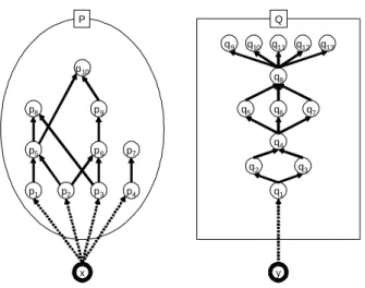
Figure 2: An example ofRdef.= ({x} ⊕P) ˙∪({y} ⊕Q).
Proof. We give a reduction from COUNTING IDEALS, that is to compute|D(P)|for a given posetP. The problem is known to be #P-complete [16]. Precisely, we consider a problem that given a posetP and an integerK ∈Z++, the query is whether or not |D(P)|< K. If we have an oracle for the query, we can compute |D(P)| by a binary search of Ks between 0 and 2|P|. We in the following give a reduction from the query if|D(P)|< K to Problem 1.
For the integer K, let Q be a poset satisfying |D(Q)|= K. The poset Q is constructed in poly(logK) time by Lemma 3.3. Let R be a poset defined by Rdef.= ({x} ⊕P) ˙∪({y} ⊕Q) (see Figure 2). Now we considerg(r) for eachr ∈R, defined by (1),
g(x) = |D(R\U(x))| = |D({y} ⊕Q)| = 1 +|D(Q)|, g(y) = |D(R\U(y))| = |D({x} ⊕P)| = 1 +|D(P)|,
g(p) = |D(R\U(p))| ≥ |D(({y} ⊕Q) ˙∪ {x})| = 2·g(x) (∀p∈P), g(q) = |D(R\U(q))| ≥ |D(({x} ⊕P) ˙∪ {y})| = 2·g(y) (∀q ∈Q),
hold. With considering the definitions (3) and (4) of the set of level idealsF(R), we obtain the following three cases;
Case 1. If |D(P)|<|D(Q)|=K, then{x} ̸∈ F(R) and {y} ∈ F(R), since g(x)> g(y).
Case 2. If |D(P)|>|D(Q)|=K, then{x} ∈ F(R) and {y} ̸∈ F(R), since g(x)< g(y).
Case 3. Otherwise, i.e. |D(P)| = |D(Q)| = K, then {x} ̸∈ F(R), {y} ̸∈ F(R), and {x, y} ∈ F(R).
Thus, if we ask the oracle for Problem 1 whether {y} ∈ F(R), then ‘yes’ (Case 1) implies
|D(P)|< K and ‘no’ (Cases 2 and 3) implies |D(P)| ≥K.
From Theorem 3.4, we observe that finding thei-th level ideal, that is Problem 2, is NP-hard even wheni= O(√
N). Precisely, we obtain the following.
Proposition 3.5 Given a poset R and an ideal S ∈ D(R), then the problem whether or not S is the ⌈√
N⌉-th LI of R is #P-hard, where N =|D(R)|.
Proof. We reduce COUNTING IDEALS to our problem. For a given poset P and K ∈ Z++, let Q and R be the posets defined in the proof of Theorem 3.4. Let N = |D(R)|, then
N = (|D(P)|+ 1)(|D(Q)|+ 1) = O(
|D(P)|2+K2)
. We define a function f :Z++ → Z++ by f(z)def.= ⌈√
z⌉.
First we show that{y}is thef(N)-th LI ofRwhenK satisfies|D(P)|< K ≤4|D(P)|. With consideringg(q)≥2g(y) for all q∈Q,{y}is thef(N)-th LI ifg(y)< f(N),f(N)≤2g(y), and f(N) ≤ g(x) hold. These conditions are transformed |D(P)|+ 1 < ⌈√
(|D(P)|+ 1)(K+ 1)
⌉
⌈√ ,
(|D(P)|+ 1)(K+ 1)
⌉≤2|D(P)|+ 2, and⌈√
(|D(P)|+ 1)(K+ 1)
⌉≤K+ 1, respectively. It is easy to see that the first and the last conditions hold when|D(P)|< K. The second condition hold ifK ≤4|D(P)|, since
⌈√(|D(P)|+ 1)(K+ 1)
⌉≤⌈√
(|D(P)|+ 1)(4|D(P)|+ 1)
⌉
<⌈√
4(|D(P)|+ 1)2
⌉= 2|D(P)|+ 2.
Next we consider the case K≤ |D(P)|, then the singleton {y} is never thef(N)-th LI ofR, sinceK ≤ |D(P)|means g(x)≤g(y), and it implies that if an LI includes y, then the LI must include x from the definition. Thus, minimizing K for which{y} is thef(N)-th LI of R, then the minimumK∗ is equal to |D(P)|+ 1.
Finally, |D(P)|is computed with checking if{y}is thef(N)-th LIs ofRfor appropriateKs, at most 2|P| times, as follows. We start from K = 2|P| and get K into halves, until{y} is the f(N)-th LI. From the above discussions, we certainly obtain the case. Suppose we get the case that {y} is the f(N)-th LI whenK =K0. In the interval [1, K0],{y} is the f(N)-th LI if, and only if, K ∈ (|D(P)|, K0]. Thus we can find K∗ = |D(P)|+ 1 according to the binary search
strategy.
With a modification of the proof of Proposition 3.5, we establish a stronger claim that finding the i-th level ideal, that is Problem 2, is #P-hard even when i = O(N1/c) for an arbitrary constantc (c≥1). Precisely, we obtain the followings.
Theorem 3.6 Suppose c (c ≥ 2) is an arbitrary constant. Given a poset R and an ideal S ∈ D(R), then the problem whether or not S is the ⌈N1/c⌉-th LI of R is #P-hard, where N =|D(R)|.
Outline of proof. We reduce COUNTING IDEALS to our problem in a similar way as the proof of Proposition 3.5. For the poset P and an arbitrary constant K, we define R′ def.= (({x} ⊕P) ˙∪({y} ⊕Q))⊕Q′, where posets Q and Q′ satisfies |D(Q)| = K and |D(Q′)| =
⌊(K+ 1)c⌋ −(K + 1)2+ 1, thus |D(R′)|= Θ(Kc). From Lemma 3.3, Q and Q′ is realized in poly(log(Kc)) = poly(logK) time and space. In a similar way as the proof of Proposition 3.5, we can show Theorem 3.6 (see Appendix A for the complete proof).
In a similar way as Theorem 3.6, we can show the #P-hardness for other functions of Ω(N1/c) and O(N), with tuning some parameters (see Appendix C).
4 Exact Computation of the poly(n)-th LI
In the previous section, we showed finding the i-th LI is #P-hard, even wheni= O(N1/c) for an arbitrary constantc ≥1. In this section, we give an exact algorithm for Problem 3, that is finding thei-th LI, which runs in time polynomial in |P|when i= O((logN)c) for an arbitrary constantc≥1.
The algorithm is essentially based on (exhaustive) enumeration of ideals of a poset. Steiner [21]
gave an enumeration algorithm for ideals of a poset, which generates all ideals one-by-one with- out duplication, and which runs in O(|P|2 +|P| · |D(P)|) time; more precisely the algorithm
Exact Algorithm
1 Input: A posetP and an integer i∈Z++. 2 For(eachp∈P){
3 Set counter Z(p) := 0.
4 Search D(P \U(p)) by an enumeration algorithmA,
with storing in counter Z(p) the number of ideals having been found.
5 if Z(p)≥ithenhalt A. 6 }
7 OutputS :={p∈P |Z(p)< i}, and halt.
Figure 3: Whole description of the exact algorithm
outputs every ideals in O(|P|) time delay, after O(|P|2) time preprocessing. Squire [20] gave a faster algorithm running in O(log|P| · |D(P)|) time.
Now we describe the algorithm for Problem 3. Let A denote an enumeration algorithm of ideals of a poset. For eachp∈P, we executeA for a posetP \U(p), and count up the number of ideals ofD(P\U(p)) one-by-one. LetZ(p) denote the value of a counter, then ifZ(p) reached atiwe haltA, and otherwiseAstops with Z(p) =|D(P\U(p))|. ThenS={p∈P |Z(p)< i} should be thei-th LI from the definition. See Figure 3 about the whole algorithm.
Clearly the time complexity of the algorithm is O(|P| · TA(i)), where TA(i) denotes the computation time in which enumeration algorithm outputs ideals up to i-th one, that is e.g., O(|P|2+|P|·i) by Steiner [21]. Thus it becomes a polynomial time algorithm wheni= poly(|P|).
In other words, Problem 3 is solvable in time polynomial in the input size wheni= O((logN)c) for an arbitrary constantc≥0, since N =|D(P)|is at most 2|P|.
5 Simple Randomized Approximation Algorithm
In this section, we give a simple randomized approximation algorithm for the i-th LI. Theo- rem 3.4 suggests that finding just a level ideal in F(P) of a given poset P is #P-hard. Thus, we consider to find an ideal S ∈ D(P), which approximates the i-th level idealSi. We use the following oracle of almost uniform sampler onD(P) for a given poset P.
Oracle 1 (Almost uniform sampler on ideals of a poset.) Given an arbitrary ε (0 < ε < 1) and a poset P, Oracle returns an element of D(P) according to a distribution ν satisfying dTV(π, ν)def.= (1/2)∥π−ν∥1 ≤ε, where π denotes the exactly uniform distribution on D(P).
Letγ1denote the time required for Oracle 1. Note that it is open whetherγ1can be poly(|P|,−lnε).
With using Oracle 1, we give the following simple randomized algorithm for Problem 2.
Algorithm 1 (ε-estimator for theλN-th LI.)
1 Input: A posetP,λ(0< λ <1),ε(0< ε≤min{λ,1−λ}), δ (0< δ <1).
2 Set Z(p) := 0 for eachp∈P.
3 Repeat(T def.= ⌈−12ε−2ln(δ/|P|)⌉ times){
4 Generate X∈ D(P) by Oracle 1 (where ν satisfies dTV(π, ν)≤ε/2).
5 For(eachp∈P){
6 if p̸∈X then Z(p) :=Z(p) + 1.
7 }
8 }
9 Set S:={p∈P |Z(p)/T < λ}. 10 OutputS and halt.
Theorem 5.1 Algorithm 1 outputs an ideal S∈ D(P) and S satisfies Pr[
S⌊(λ−ε)N⌋⊆S ⊆S⌈(λ+ε)N⌉]
≥1−δ, (5)
in O((γ1+|P|) log(|P|)ε−2logδ−1) time.
Proof. The time complexity is easy to see. First we show that the output S of Algorithm 1 is an ideal of P. Suppose a pair p ∈P and q ∈P satisfies p ≺q. We show that ifq ∈ S then p∈S. For any random sample X∈ D(P) in Step 1, ifq∈X thenp∈X, since X is an ideal of P. It implies Z(p) ≥Z(q) in Step 1. Thus ifq ∈S then p∈S from the definition of S in Step 2.
Next, to show that S satisfies the inequality (5), we establish the following.
Claim. For any p∈P,
Case 1. if g(p)≤(λ−ε)N, then the probability p̸∈S (i.e., Z(p)/T ≥λ) is at most δ/|P|, and Case 2. if g(p)≥(λ+ε)N, then the probability p∈S (i.e., Z(p)/T < λ) is at most δ/|P|. We define ωp
def.= g(p)/N forp∈P. Let ωbp be an estimator ofωp by the distribution ν, that is formally defined by
b
ωp def.= ∑
X∈D(P)|p̸∈X
ν(X).
In Case 1,p∈P satisfiesg(p)/N ≤λ−ε, thenωp+ε≤λholds. Now, with considering that the distributionν satisfiesdTV(π, ν)≤ε/2, we have ωbp ≤ωp+ε/2, that implies ωbp+ε/2≤ωp+ε.
Thus we obtainωbp+ε/2≤λ. Then the probability Z(p)/T ≥λsatisfies that Pr [Z(p)≥λT] ≤ Pr
[
Z(p)≥( b ωp+ ε
2 )
T ]
= Pr [
Z(p)≥ (
1 + ε 2bωp
) b ωp·T
] .
By using the Chernoff’s bound,
Pr [
Z(p)≥ (
1 + ε 2ωbp
) b ωp·T
]
≤ e
−1 3ωbpT
( ε 2bωp
)2
= e
− ε2 12bωp
T ≤ δ
|P| where we use T =⌈−12ε−2ln(δ/|P|)⌉. We obtain the claim in Case 1.
In a similar way, we obtain Case 2. From the assumption of the case, ωp −ε ≥ λ. Since dTV(π, ν) ≤ ε/2, we have ωbp ≥ ωp −ε/2, that implies ωbp −ε/2 ≥ ωp −ε. Thus we obtain b
ωp−ε/2≥λ. Then
Pr [Z(p)< λT] ≤ Pr [
Z(p)<
(bωp− ε 2 )
T ]
= Pr [
Z(p)<
( 1− ε
2bωp
) b ωp·T
] .
By using the Chernoff’s bound,
Pr [
Z(p)<
( 1− ε
2bωp
) b ωp·T
]
≤ e
−1 2bωpT
( ε 2ωbp
)2
= e
− ε2 8ωbpT
≤ δ
|P| where we use T def.= ⌈−12ε−2ln(δ/|P|)⌉. We obtain Claim.
We conclude the proof by showing that S satisfies the inequality (5). If S(λ−ε)N ̸⊆S, then there exists a p ∈ S(λ−ε)N and p ̸∈ S. It implies that if S(λ−ε)N ̸⊆ S, then there exists a p∈ P satisfying that g(p) <(λ−ε)N and Z(p)/T ≥λ. From Case 1 of the above Claim, the probability ofS(λ−ε)N ̸⊆S satisfies that
Pr[
S(λ−ε)N ̸⊆S]
≤ ∑
p∈S(λ−ε)N
Pr[p̸∈S] ≤ |{p|g(p)<(λ−ε)N}| · δ
|P|.
In a similar way, if S ̸⊆ S(λ+ε)N, then there exists a p̸∈ S(λ+ε)N and p ∈S. It implies that if S ̸⊆S(λ+ε)N, then there exists a p∈P satisfying that g(p)≥(λ+ε)N and Z(p)/T < λ. From Case 2 of the above Claim, the probability ofS ̸⊆S(λ+ε)N satisfies that
Pr[
S̸⊆S(λ+ε)N]
≤ ∑
p̸∈S(λ+ε)N
Pr[p∈S] ≤ |{p|g(p)≥(λ+ε)N}| · δ
|P|.
Since the sets {p|g(p)<(λ−ε)N} and{p|g(p)≥(λ+ε)N} are disjoint, we obtain Pr[
S(λ−ε)N ⊆Z ⊆S(λ+ε)N]
≥ 1− |P| · δ
|P| = 1−δ.
6 Randomized Approximation Based on Counting Ideals
The time complexity of Algorithm 1, in the previous section, gets larger proportional toε−2. As we showed in Section 3, Problem 2 is #P-hard even wheniis small as fractional power ofN. For smalli, we have to setεin Algorithm 1 very small asε≤i/N, it makes Algorithm 1 inefficient.
In this section, we propose another approximation algorithm for the i-th LI, especially for a smalli. The algorithm approximately computesg(p) for eachp∈P. Then, we use the following oracle.
Oracle 2 (RAS for COUNTING IDEALS.) Given an arbitrary ε (0 < ε <1), δ (0< δ <1), and a posetP, Oracle returns Z∈Z+ which approximates |D(P)|satisfying
Pr
[|Z− |D(P)||
|D(P)| ≤ε ]
≥1−δ.
Letγ2denote the time required for Oracle 2. Oracle 2 is obtained from Oracle 1 in poly(ε−1,−lnδ,|P|, γ1) time, more precisely O(γ1|P|2ε−2ln(|P|/δ)) with using aself-reducibility. See e.g. [10] about a
relationship between sampling and approximate counting.
An essential idea of approximation algorithm for thei-th LI is to compute an estimatorbg(p) forg(p) for everyp∈P, and to find a setS ⊆P satisfyingg(p)b < k. Unfortunately, this simple idea cannot find an ideal S ∈ D(P), since an event of bg(p)< k ≤bg(q) happen to a pair p≺q with a non-negligible probability. The following algorithm gets rid of this issue.
Algorithm 2 (ε-estimator for thef(N)-th LI.)
1 Input: A posetP,ε(0< ε < λ), δ (0< δ <1), a function3 f :Z++→Z++. 2 Compute Nb approximating|D(p)|by Oracle 2.
3 Set k=f(Nb)
(wherek satisfies4 Pr[|k− |f(N)|| ≤(ε/3)· |f(N)|]≥1−δ/(2|P|)).
4 Set S:=∅.
5 While(∃p∈P \S, s.t. q∈S (∀q≺p)){
6 Computebg(p) approximatingg(p) by Oracle 2
(where bg(p) satisfies Pr [|bg(p)−g(p)| ≤(ε/3)·g(p)]≥1−δ/(2|P|)).
7 If bg(p)< k thenS :=S∪ {p}. 8 }
9 OutputS and halt.
Theorem 6.1 Algorithm 2 outputs an ideal S∈ D(P) and S satisfies Pr[
S⌊(1−ε)·f(N)⌋⊆S⊆S⌈(1+ε)·f(N)⌉]
≥1−δ in O(|P|γ2) time.
Proof of Theorem 6.1. The time complexity is easy to see. It is also easy to see that an output of Algorithm 2 is an ideal ofP, sincep∈Simplies that Algorithm 2 computedbg(p), that is only whenq∈P (∀q≺p). We show thatS satisfies the inequality (6). From the condition of Algorithm 2, ksatisfies
Pr
[|k−f(N)|
f(N) > ε 3 ]
< δ 2|P|. Then we obtain the following.
Claim 1 The probability thatk >(1 +ε/3)·f(N) or k <(1−ε/3)·f(N) is less thanδ/(2|P|).
Suppose we have values bg(p) for all p∈P, satisfying Pr
[|bg(p)−g(p)| g(p) ≤ ε
3 ]
≥1− δ
2|P|, (6)
and bg(p) coincident to the values in Algorithm 2 if it is computed. We show the following;
Claim 2 For any p∈P,
Case 1. if g(p)≥(1 +ε)·f(N), the probability bg(p)≤(1 + (1/3)ε)·f(N) is less thanδ/(2|P|), and
Case 2. if g(p)≤(1−ε)·f(N), the probability bg(p)≥(1−(1/3)ε)·f(N) is less thanδ/(2|P|).
In Case 1, from Inequation (6), with a probability at least 1−δ/(2|P|), b
g(p) ≥ (
1−1 3ε
)
·g(p) ≥ (
1−1 3ε
)
·(1 +ε)·f(N)
≥ (
1 +2−ε 3 ε
)
·f(N) >
( 1 +1
3ε )
·f(N) hold. In Case 2, from Inequation (6), with a probability at least 1−δ/(2|P|),
b g(p) ≤
( 1 +1
3ε )
·g(p) ≤ (
1 +1 3ε
)
·(1−ε)·f(N)
≤ (
1−2 +ε 3 ε
)
·f(N) <
( 1−1
3ε )
·f(N) hold. We obtain the claim.
From Claim 1 and 2, we obtain the following (see Figure 4);
4We naturally assume that the function is a contraction mapping and nondecreasing, e.g., ⌊√
z⌋, ⌈z1/c⌉,
⌈log(z)⌉, etc.
4If the function f is a contraction mapping and nondecreasing, the condition is satisfied whenNb satisfies Pr[|Nb− |D(p)|| ≤(ε/3)· |D(p)|]≥1−δ/(2|P|).
-
(1 ")f(N) 1
"
3
f(N) f(N) 1+
"
3
f(N) (1+")f(N) thenbn(p)< 1
"
3
f(N),
w.p. 1 Æ
2jPj
thenbn(p)> 1+
"
3
f(N),
w.p. 1 Æ
2jPj
ksatisesthat,
1
"
3
f(N)k 1+
"
3
f(N),
w.p. 1 Æ
2jPj Æ
Æ
-
-
Figure 4: A figure of the relationship betweenk and bg(p).
Claim 3 For any p∈P,
Case 1. if g(p)≥(1 +ε)·f(N), then g(p)b < k with a probability less thanδ/|P|, and Case 2. if g(p)≤(1−ε)·f(N), then g(p)b ≥k with a probability less thanδ/|P|.
Now we conclude the proof by showing (6). Algorithm 2 implies that ifS(1−ε)·f(N)̸⊆S, then there exists a p ∈ P satisfying g(p) <(1−ε)·f(N), and exists a q ∈ P satisfying q ≺p and b
g(q)< k. Note thatq ≺p meansg(q)< g(p), thus the above claim can be simply transformed into that if S(1−ε)·f(N) ̸⊆ S, then there exists a q ∈ P satisfying g(q) < (1−ε)·f(N) and b
g(q)< k. From Case 1 of Claim 3, the probability ofS(1−ε)·f(N)̸⊆S satisfies that Pr[
S(1−ε)·f(N)̸⊆S]
≤ ∑
p∈S(1−ε)·f(N)
Pr[p̸∈S]
≤ |{p|g(p)<(1−ε)·f(N)}|· δ
|P|.
In a similar way, ifS ̸⊆S(1+ε)·f(N), then there exists ap̸∈S(1+ε)·f(N)and p∈S. It implies that ifS̸⊆S(1+ε)·f(N), theng(p)≥(1 +ε)·f(N) andg(p). From Case 2 of Claim 3, the probabilityb of S̸⊆S(1+ε)·f(N) satisfies that
Pr[
S̸⊆S(1+ε)·f(N)]
≤ ∑
p̸∈S(1+ε)·f(N)
Pr[p∈S]
≤ |{p|g(p)≥(1 +ε)·f(N)}|· δ
|P|.
Since the sets {p|g(p)<(1−ε)·f(N)} and {p|g(p)≥(1 +ε)·f(N)} are disjoint, we obtain Pr[
S(1−ε)·f(N) ⊆Z ⊆S(1+ε)·f(N)]
≥ 1− |P| · δ
|P| = 1−δ.
7 Concluding Remarks
We gave randomized approximation schemes for thei-th GMSM using an almost uniform sampler on ideals of a poset. The existence of a polynomial time almost uniform sampler on ideals (or antichains) of a poset, or an FPRAS for counting, is open. Note that conversely if we have a fully polynomial-time randomized approximation scheme for the i-th GMSM in a form
such as Theorem 5.1 or 6.1, then we can obtain an FPRAS for counting ideals of a poset (see Appendix D), and hence a polynomial time almost uniform sampler (see e.g. [10]).
In case that a rotation poset belongs to some special classes such as series-parallel, bounded width, etc., then we can find thei-th GMSM exactly in polynomial time by Steiner’s result [22].
No results seem to be known on a characterization of preference lists whose rotation posets belongs to such classes of polynomial time solvable, as far as we see. It is also open whether or not Problems 1 and 2 are in NP.
Acknowledgment
The authors thank Professor Shin-Ichi Nakano for his helpful comment. The first author is supported by Grant-in-Aid for Scientific Research.
References
[1] N. Bhatnagar, S. Greenberg, and D. Randall, Sampling stable marriages: why the spouse- swapping won’t work, Proceedings of the nineteenth annual ACM-SIAM symposium on Discrete algorithms (SODA 2008), 1223–1232.
[2] C. Blair, Every finite distributive lattice is a set of stable matchings, Journal of Combina- torial Theory A,37 (1984), 353–356.
[3] C.T. Cheng, The generalized median stable matchings: finding them is not that easy, Proceedings of the 8th Latin American Theoretical Informatics (Latin 2008), 568–579.
[4] B.A. Davey and H.A. Priestley, Introduction to Lattices and Order, Second Edition, Cam- bridge University Press, 2002.
[5] D.P. Dubhashi, K. Mehlhorn, D. Rajan, and C.Thiel, Searching, sorting and randomised algorithms for central elements and ideal counting in posets, Lecture Notes in Computer Science,761 (1993), 436–443 .
[6] D. Gale and L.S. Shapley, College admissions and the stability of marriage, The American Mathematics Monthly, 69(1962), 9–15.
[7] M.R. Garey and D.S. Johnson, A Guide to the Theory of NP-Completeness, W. H. Freeman, 1979.
[8] D. Gusfield and R.W. Irving, The Stable Marriage Problem, Structure and Algorithms, The MIT Press, 1989.
[9] R.W. Irving and P. Leather, The complexity of counting stable marriages, SIAM Journal on Computing,15 (1986), 655–667.
[10] M. Jerrum, Counting, Sampling and Integrating: Algorithms and Complexity, ETH Z¨urich, Birkhauser, Basel, 2003.
[11] B. Klaus and F. Klijn, Median stable matching for college admission, International Journal of Game Theory,34(2006), 1–11.
[12] B. Klaus and F. Klijn, Smith and Rawls share a room: stability and medians, Meteor RM/08-009 (2008), Maastricht University,
http://edocs.ub.unimaas.nl/loader/file.asp?id=1307
[13] D. Knuth, Stable Marriage and Its Relation to Other Combinatorial Problems, American Mathematical Society, 1991.
[14] T. Nemoto, Some remarks on the median stable marriage problem, Proceedings of 17th International Symposium on Mathematical Programming, 2000.
[15] J. Propp and D.B.Wilson, Exact sampling with coupled Markov chains and applications to statistical mechanics, Random Structures and Algorithms,9 (1996), 223–252.
[16] J.S. Provan and M.O. Ball, The complexity of counting cuts and of computing the proba- bility that a graph is connected, SIAM Journal on Computing,12(1983), 777–788.
[17] A.E. Roth and M.A.O. Sotomayor, A. Two-Sided Matchings: A Study In Game-Theoretic Modeling And Analysis, Cambridge University Press, 1990.
[18] M. Schwarz and M.B. Yenmez, Median stable matching, 2007, available at SSRN;
http://ssrn.com/abstract=1031277
[19] J. Sethuraman, C.P. Teo, and L. Qian, Many-to one stable matching: geometry and fairness, Mathematics of Operations Research,31(2006), 581–596.
[20] M.B. Squire, Enumerating the ideals of a poset, preprint, North Carolina State University, 1995.
[21] G. Steiner, An algorithm for generating the ideals of a partial order, Operations Research Letters,5 (1986), 317–320.
[22] G. Steiner, On the complexity of dynamic programming for sequencing problems with precedence constraints, Annals of Operations Research,26(1990), 103–123.
[23] C.P. Teo and J. Sethuraman, The geometry of fractional stable matchings and its applica- tions, Mathematics of Operations Research, 23(1998), 874–891.
A Proof of Theorem 3.6
Theorem 3.6. Suppose c (c ≥ 2) is an arbitrary constant. Given a poset R and an ideal S ∈ D(R), then the problem whether or not S is the ⌈N1/c⌉-th LI of R is #P-hard, where N =|D(R)|.
Proof. We reduce COUNTING IDEALS for a given poset P to our problem in a similar way as the proof of Proposition 3.5. For the poset P and an arbitrary positive integer K, we define R′ def.= (({x} ⊕P) ˙∪({y} ⊕Q))⊕Q′, where posets Q and Q′ satisfies |D(Q)| = K and |D(Q′)| = ⌊(K + 1)c⌋ −(K + 1)2 + 1. From Lemma 3.3, Q and Q′ is constructible in poly(log(Kc)) = poly(logK) time and space. Let N =|D(R′)|, then N =⌊(K+ 1)c⌋ −(K + 1)2+ (|D(P)|+ 1)(K+ 1). We define a function f :Z++→Z++ by f(z)def.= ⌈z1/c⌉, then
f(N) = ⌈(
⌊(K+ 1)c⌋ −(K+ 1)2+ (|D(P)|+ 1)(K+ 1))1/c⌉
=
⌈(⌊(K+ 1)c⌋+ (|D(P)| −K)(K+ 1))1/c
⌉
. (7)
For eachr ∈R′,g(r), that is defined by (1), satisfies g(x) = |D({y} ⊕Q)| = |D(Q)|+ 1, g(y) = |D({x} ⊕P)| = |D(P)|+ 1,
g(p) ≥ |D(({x} ⊕P) ˙∪ {y})| = 2·g(x) (∀p∈P), g(q) ≥ |D(({y} ⊕Q) ˙∪ {x})| = 2·g(y) (∀q ∈Q), g(q′) ≥ g(q) ≥ 2·g(y) (∀q′ ∈Q′).
Now we show that{y}is thef(N)-th LI ofRwhenKsatisfies|D(P)|< K ≤2|D(P)|. With considering g(q) ≥ 2·g(y) for all q ∈Q, {y} is the f(N)-th LI if g(y) < f(N), f(N) ≤ 2g(y), and f(N)≤g(x) hold. These conditions are transformed with (7) into
|D(P)|+ 1<
⌈
(⌊(K+ 1)c⌋+ (|D(P)| −K)(K+ 1))1/c
⌉
, (8)
⌈
(⌊(K+ 1)c⌋+ (|D(P)| −K)(K+ 1))1/c
⌉≤2|D(P)|+ 2, (9)
⌈
(⌊(K+ 1)c⌋+ (|D(P)| −K)(K+ 1))1/c
⌉≤K+ 1, (10)
respectively. It is easy to see that the condition (10) hold if |D(P)| < K. We show that the condition (8) hold if |D(P)|< K. With considering that
f(N) =
⌈
(⌊(K+ 1)c⌋+ (|D(P)| −K)(K+ 1))1/c
⌉
≥ ⌈
((K+ 1)c−1 + (|D(P)| −K)(K+ 1))1/c
⌉
≥ ((K+ 1)c−1 + (|D(P)| −K)(K+ 1))1/c,
it is enough to show that (K + 1)c −1 + (|D(P)| −K)(K + 1)−(|D(P)|+ 1)c > 0 when
|D(P)|+ 1≤K and c≥2. Then, with the following transformations (K+ 1)c−1 + (|D(P)| −K)(K+ 1)−(|D(P)|+ 1)c
= (K+ 1)c−(|D(P)|+ 1)c+ (|D(P)| −K)(K+ 1)−1
≥ (K+ 1)⌊c⌋−(|D(P)|+ 1)⌊c⌋+ (|D(P)| −K)(K+ 1)−1