RIMS-1721
Computing the Maximum Degree of Minors in
Mixed Polynomial Matrices via Combinatorial Relaxation
By
Satoru IWATA and Mizuyo TAKAMATSU
May 2011
R ESEARCH I NSTITUTE FOR M ATHEMATICAL S CIENCES
KYOTO UNIVERSITY, Kyoto, Japan
Computing the Maximum Degree of Minors in
Mixed Polynomial Matrices via Combinatorial Relaxation
∗Satoru Iwata† Mizuyo Takamatsu‡ May 6, 2011
Abstract
Mixed polynomial matrices are polynomial matrices with two kinds of nonzero coeffi- cients: fixed constants that account for conservation laws and independent parameters that represent physical characteristics. The computation of their maximum degrees of minors is known to be reducible to valuated independent assignment problems, which can be solved by polynomial numbers of additions, subtractions, and multiplications of rational functions.
However, these arithmetic operations on rational functions are much more expensive than those on constants.
In this paper, we present a new algorithm of combinatorial relaxation type. The algo- rithm finds a combinatorial estimate of the maximum degree by solving a weighted bipartite matching problem, and checks if the estimate is equal to the true value by solving indepen- dent matching problems. The algorithm mainly relies on fast combinatorial algorithms and performs numerical computation only when necessary. In addition, it requires no arithmetic operations on rational functions. As a byproduct, this method yields a new algorithm for solving a linear valuated independent assignment problem.
1 Introduction
Let A(s) = (Aij(s)) be a rational function matrix with Aij(s) being a rational function in s.
The maximum degree δk(A) of minors of orderk is defined by δk(A) = max{deg detA[I, J]| |I|=|J|=k},
where degf denotes the degree of a rational function f(s), andA[I, J] denotes the submatrix with row setI and column setJ. Thisδk(A) determines the Smith-McMillan form at infinity of a rational function matrix [27], which is used in decoupling and disturbance rejection of linear
∗A preliminary version of this paper is to appear in Proceedings of the 15th Conference on Integer Program- ming and Combinatorial Optimization.
†Research Institute for Mathematical Sciences, Kyoto University, Kyoto 606-8502, Japan. Supported by a Grant-in-Aid for Scientific Research from the Japan Society for Promotion of Science. E-mail:
‡Department of Information and System Engineering, Chuo University, Tokyo 112-8551, Japan. Sup- ported by a Grant-in-Aid for Scientific Research from the Japan Society for Promotion of Science. E-mail:
time-invariant systems, and the Kronecker canonical form of a matrix pencil [4, 7, 26], which is used in analysis of linear DAEs with constant coefficients. Thus, the computation of δk(A) is a fundamental and important procedure in dynamical systems analysis.
The notion of mixed polynomial matrices [15, 22] was introduced as a mathematical tool for faithful description of dynamical systems such as electric circuits, mechanical systems, and chemical plants. A mixed polynomial matrix is a polynomial matrix that consists of two kinds of coefficients as follows.
Accurate Numbers (Fixed Constants) Numbers that account for conservation laws are precise in values. These numbers should be treated numerically.
Inaccurate Numbers (Independent Parameters) Numbers that represent physical char- acteristics are not precise in values. These numbers should be treated combinatorially as nonzero parameters without reference to their nominal values. Since each such nonzero entry often comes from a single physical device, the parameters are assumed to be inde- pendent.
For example, physical characteristics in engineering systems are not precise in values because of measurement noise, while exact numbers do arise in conservation laws such as Kirchhoff’s conservation laws in electric circuits, or the law of conservation of mass, energy, or momentum and the principle of action and reaction in mechanical systems. Thus, it is natural to distinguish inaccurate numbers from accurate numbers in the description of dynamical systems.
In [21], Murota reduces the computation of δk(A) for a mixed polynomial matrixA(s) to solving avaluated independent assignment problem, for which he presents in [19, 20] algorithms that perform polynomial numbers of additions, subtractions, and multiplications of rational functions. However, these arithmetic operations on rational functions are much more expensive than those on constants.
In this paper, we present an algorithm for computing δk(A), based on the framework of
“combinatorial relaxation.” The outline of the algorithm is as follows.
Phase 1 Construct a relaxed problem by discarding numerical information and extracting zero/nonzero structure inA(s). The solution is regarded as an estimate ofδk(A).
Phase 2 Check whether the obtained estimate is equal to the true value of δk(A), or not. If it is, return the estimate and halt.
Phase 3 Modify the relaxation so that the invalid solution is eliminated, and find a solution to the modified relaxed problem. Then go back to Phase 2.
In this algorithm, we solve a weighted bipartite matching problem in Phase 1 and indepen- dent matching problems in Phase 2. We remark that our algorithm does not need symbolic operations on rational functions.
This framework of combinatorial relaxation algorithm is somewhat analogous to the idea of relaxation and cutting plane in integer programming. In contrast to integer programming, where hard combinatorial problems are relaxed to linear programs, here we relax a linear algebraic problem to an efficiently solvable combinatorial problem. Then the algorithm checks
the validity of the obtained solution and modifies the relaxation if necessary just like adding a cutting plane. This is where the name “combinatorial relaxation” comes from. See [22, §7.1]
for more details.
We now summarize previous works based on the framework of combinatorial relaxation.
The combinatorial relaxation approach was invented by Murota [16] for computing the Newton polygon of the Puiseux series solutions to determinantal equations. This approach was further applied to the computation of the degree of detA(s) in [17] and δk(A) in [9, 10, 11, 18] for a polynomial matrixA(s). In computational efficiency of the algorithms, it is crucial to solve the relaxed problem efficiently and not to invoke the modification of the relaxation many times. The result in [11] shows practical efficiency of the combinatorial relaxation through computational experiments.
Let us have a closer look at the algorithms [9, 10, 11, 18] for δk(A). In [18], Murota presented a combinatorial relaxation algorithm for general rational function matrices using biproper equivalence transformations in the modification of the relaxed problem. The primal- dual version was presented in [11]. These algorithms need to transform a polynomial matrix by row/column operations, which possibly increase the number of terms in some entries. To avoid this phenomenon in the case of matrix pencils, Iwata [9] presented another combinatorial relaxation algorithm, which uses only strict equivalence transformations.
Another approach presented in [10] uses a mixed polynomial matrix as a combinatorial relaxation. Given a mixed polynomial matrix, one can compute the maximum degree of minors by solving a valuated independent assignment problem. When specific values are assigned into the independent parameters, the maximum degree of minors may change. The combinatorial relaxation algorithm in [10] computes the resulting exact value.
In this paper, we extend the combinatorial relaxation framework to mixed polynomial matrices. In contrast to the previous work [10], our goal is to compute the maximum degree of minors in a given mixed polynomial matrix efficiently. Our combinatorial relaxation is the assignment problem obtained by replacing accurate numbers by independent parameters. Our algorithm adopts a different way of matrix modification from the previous algorithms [10, 11, 18], which enables us to evaluate the complexity by the number of basic arithmetic operations.
For anm×nmixed polynomial matrix withm≤n, the algorithm runs inO(mω+1nd2max) time, whereω is the matrix multiplication exponent anddmax is the maximum degree of an entry.
We compare this time complexity with that of the previous algorithm of Murota [21] based on the valuated independent assignment. The bottleneck in that algorithm is to transform an m×n polynomial matrix into an upper triangular matrix in each iteration. This can be done inO~(mωndmax) time, whereO~indicates that we ignore log(mdmax) factors, by using Bareiss’
fraction-free Gaussian elimination approach [1, 2, 25] and anO(dlogdlog logd) time algorithm in [3] for multiplying polynomials of degree d. Since the number of iterations is k, Murota’s algorithm runs in O~(kmωndmax) time. Thus the worst-case complexity of our algorithm is comparable to that of the previous one.
However, our combinatorial relaxation algorithm terminates without invoking the modifi- cation of the relaxation unless there is an unlucky numerical cancellation. Consequently, in most cases, it runs in O(mωndmax) time, which is much faster than the previous algorithm.
One application of our combinatorial relaxation algorithm is to compute the Kronecker
canonical form of a mixed matrix pencil, which is a mixed polynomial matrix with dmax = 1.
For an n×nregular mixed matrix pencil, our algorithm enables us to compute the Kronecker canonical form in O(nω+2) time. This time complexity is better than the previous algorithm given in [12], which makes use of another characterization based on expanded matrices.
Another application is to compute the optimal value of a linear valuated independent assign- ment problem. The optimal value of this problem coincides with the degree of the determinant of an associated mixed polynomial matrix. Thus we can make use of our combinatorial relax- ation algorithm. This means that we find the optimal value of a linear valuated independent assignment problem by solving a sequence of independent matching problems.
Combinatorial relaxation approach exploits the combinatorial structures of polynomial ma- trices and exhibits a connection between combinatorial optimization and matrix computation.
While recent works of Mucha and Sankowski [13, 14], Sankowski [24], and Harvey [8] utilize matrix computation to solve matching problems, this paper adopts the opposite direction, that is, we utilize matching problems for matrix computation.
The organization of this paper is as follows. Section 2 is devoted to preliminaries on rational function matrices, the independent matching problem, and mixed matrix theory. We present a combinatorial relaxation algorithm in Section 3, and analyze its complexity in Section 4. In Section 5, we apply the combinatorial relaxation approach to the linear valuated independent assignment problem.
2 Preliminaries
We provide preliminaries on rational functions (Section 2.1), independent matching problems (Section 2.2), and mixed polynomial matrices (Section 2.3). Then we explain how to reduce the computation of the rank of a layered mixed matrix to an independent matching problem in Section 2.4.
2.1 Rational Function Matrices
We denote the degree of a polynomial g(s) by degg, where deg 0 = −∞ by convention. For a rational function f(s) =g(s)/h(s) with polynomials g(s) and h(s), its degree is defined by degf = degg−degh. A rational functionf(s) is calledproper if degf ≤0, andstrictly proper if degf < 0. We call a rational function matrix (strictly) proper if its entries are (strictly) proper rational functions. A square proper rational function matrix is called biproper if it is invertible and its inverse is a proper rational function matrix. A proper rational function matrix is biproper if and only if its determinant is a nonzero constant. It is known that δk(A) is invariant under biproper equivalence transformations, i.e.,
δk(A) =δk( ˜A) (k= 1, . . . ,rankA(s)) if ˜A(s) =U(s)A(s)V(s) with biproper matricesU(s) and V(s).
A rational function matrixZ(s) is called aLaurent polynomial matrixifsKZ(s) is a polyno- mial matrix for some integerK. In our algorithm, we make use of biproper Laurent polynomial matrices in the phase of matrix modification.
2.2 Independent Matching Problem
A matroid is a pair M= (V,I) of a finite setV and a collectionI of subsets of V such that (I-1) ∅ ∈ I,
(I-2) I ⊆J ∈ I ⇒I ∈ I,
(I-3) I, J ∈ I,|I|<|J| ⇒I∪ {v} ∈ I for somev∈J\I.
The setV is called theground set,I ∈ I is anindependent set, andIis thefamily of independent sets. The following problem is an extension of the matching problem.
[Independent Matching Problem (IMP)]
Given a bipartite graph G = (V+, V−;E) with vertex sets V+, V− and edge set E, and a pair of matroids M+ = (V+,I+) and M− = (V−,I−), find a matching M ⊆E that maximizes|M|subject to
∂+M ∈ I+, ∂−M ∈ I−, (1) where ∂+M and ∂−M denote the set of vertices in V+ and V− incident to M, respectively.
A matchingM ⊆E satisfying (1) is called anindependent matching.
2.3 Mixed Matrices and Mixed Polynomial Matrices
A generic matrix is a matrix in which each nonzero entry is an independent parameter. A matrix A is called a mixed matrix ifA is given by A =Q+T with a constant matrix Q and a generic matrix T. A layered mixed matrix (or an LM-matrix for short) is defined to be a mixed matrix such thatQandT have disjoint nonzero rows. An LM-matrixAis expressed by A=(Q
T
).
A polynomial matrix A(s) is called a mixed polynomial matrix if A(s) is given by A(s) = Q(s) +T(s) with a pair of polynomial matricesQ(s) =∑N
k=0skQkandT(s) =∑N
k=0skTkthat satisfy the following two conditions.
(MP-Q) Qk (k= 0,1, . . . , N) are constant matrices.
(MP-T) Tk (k= 0,1, . . . , N) are generic matrices.
A layered mixed polynomial matrix (or an LM-polynomial matrix for short) is defined to be a mixed polynomial matrix such that Q(s) and T(s) have disjoint nonzero rows. An LM- polynomial matrix A(s) is expressed byA(s) =(Q(s)
T(s)
). The matrix A(s) =(Q(s)
T(s)
) is called anLM-Laurent polynomial matrix if sKA(s) is an LM- polynomial matrix for some integerK. We denote the row set and the column set ofA(s) byR andC, and the row sets of Q(s) andT(s) byRQ andRT. We also setmQ=|RQ|,mT =|RT|, and n = |C| for convenience. The (i, j) entry of Q(s) and T(s) is denoted by Qij(s) and Tij(s), respectively. We use these notations throughout this paper for LM-Laurent polynomial
matrices as well as LM-matrices. For an LM-Laurent polynomial matrix A(s) =(Q(s)
T(s)
), let us define
δkLM(A) ={deg detA[RQ∪I, J]|I ⊆RT, J ⊆C,|I|=k,|J|=mQ+k},
where 0≤k≤min(mT, n−mQ). Note thatδkLM(A) designates the maximum degree of minors of ordermQ+kwith row set containing RQ.
We denote an m×mdiagonal matrix with the (i, i) entry beingai by diag[a1, . . . , am]. Let A(s) = ˜˜ Q(s) + ˜T(s) be anm×nmixed polynomial matrix with row setR and column set C.
We construct a (2m)×(m+n) LM-polynomial matrix A(s) =
(
diag[sd1, . . . , sdm] Q(s)˜
−diag[t1sd1, . . . , tmsdm] T(s)˜ )
, (2)
where ti(i= 1, . . . , m) are independent parameters and di = maxj∈Cdeg ˜Qij(s) for i ∈R. A mixed polynomial matrix ˜A(s) and its associated LM-polynomial matrixA(s) have the following relation, which implies that the value ofδk( ˜A) is obtained fromδLMk (A).
Lemma 2.1 ([22, Lemma 6.2.6]). Let ˜A(s) be an m×n mixed polynomial matrix and A(s) the associated LM-polynomial matrix defined by (2). Then it holds that
δk( ˜A) =δLMk (A)−
∑m i=1
di.
2.4 Rank of LM-matrices
The computation of the rank of an LM-matrix A=(Q
T
) is reduced to solving an independent matching problem [23] as follows. See [22,§4.2.4] for details.
Let CQ = {jQ |j ∈ C} be a copy of the column set C of A. Consider a bipartite graph G= (V+, V−;ET ∪EQ) withV+ =RT ∪CQ,V−=C,
ET ={(i, j)|i∈RT, j ∈C, Tij = 0̸ } and EQ ={(jQ, j)|j∈C}. LetM+= (V+,I+) be a matroid defined by
I+={I+⊆V+|rankQ[RQ, I+∩CQ] =|I+∩CQ|}, and M− be a free matroid. Then rankA has the following property.
Theorem 2.2 ([22, Theorem 4.2.18]). LetA be an LM-matrix. Then the rank of A is equal to the maximum size of an independent matching in the problem defined above, i.e.,
rankA= max{|M| |M : independent matching}.
We describe the algorithm [22] for computing rankA as follows. Let us denote the reori- entation of a ∈ ET ∪EQ by a◦. With reference to G and an independent matching M, we
construct an auxiliary graphGM = ( ˜V ,E) with ˜˜ V =V+∪V− and ˜E =ET ∪EQ∪E+∪M◦, where
E+ ={(i, j)|i∈∂+M∩CQ, j ∈CQ\∂+M, ∂+M \ {i} ∪ {j} ∈ I+}, M◦ ={a◦|a∈M}.
Let I0 be any subset of C satisfying rankQ[RQ, I0] = rankQ. We determine an initial independent matching by using I0.
Algorithm for the Rank of an LM-matrix
Step 1 M ← {(jQ, j)|j∈I0}. Then we transformQby row operations so thatQ[RQ, ∂+M∩ CQ] is in the form of(D
O
) withDbeing a diagonal matrix.
Step 2 If there exists inGM = ( ˜V ,E) a directed path from˜ S+=RT\∂+MtoS−=C\∂−M, then go to Step 3. Otherwise output rankA=|M|and halt.
Step 3 LetP be a shortest path from S+ toS−. M ←(M \ {a∈M |a◦ ∈P ∩M◦})∪(P ∩ ET)∪(P∩EQ). Then we transformQby row operations so thatQ[RQ, ∂+M∩CQ] is in the form of(D
O
) withDbeing a diagonal matrix. Go to Step 2.
Let ˜A=(Q˜ T˜
) be an LM-matrix obtained at the termination of this algorithm. Then we have (Q˜
T˜ )
= (
U O O I
) ( Q T
)
(3) for some nonsingular constant matrix U, because Q is transformed into ˜Q by row operations in Steps 1 and 3.
The structure of an LM-matrix ˜A = ( ˜Aij) is represented by a bipartite graph G( ˜A) = (RQ∪RT, C;E( ˜A)) with E( ˜A) = {(i, j) |i ∈ RQ∪RT, j ∈ C,A˜ij ̸= 0}. The maximum size of a matching in G( ˜A) is called the term-rank of ˜A, denoted by term-rank ˜A. Now ˜A has the following property, which forms the basis of the algorithm to compute the combinatorial canonical form (CCF) of an LM-matrix [22,§4.4].
Lemma 2.3. Let ˜A be an LM-matrix obtained at the termination ofAlgorithm for the Rank of an LM-matrix. Then we have rank ˜A= term-rank ˜A.
Proof. For ˜A=(Q˜ T˜
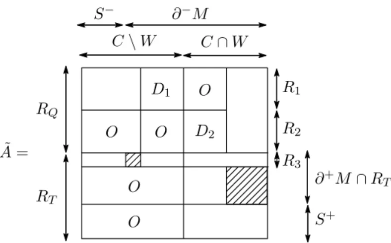
), we denote the row sets of ˜Q and ˜T by RQ and RT, and the column set of A˜ by C. We may assume that ˜Ais of full row rank, because the rows consisting only of zeros can be ignored. Let W be the set of vertices reachable from S+ in GM at the termination of the algorithm. Since there is no directed path fromS+ toS−, it holds thatS−⊆C\W. Hence C∩W ⊆∂−M follows fromS−=C\∂−M.
We put B = {j ∈ C | jQ ∈ ∂+M ∩CQ}. Then ˜A[RQ, B] is expressed as ˜A[RQ, B] = (
D1 O O D2
)
, where D1 and D2 are diagonal matrices with column sets B1 ⊆ C \W and B2 ⊆C∩W. The row sets ofD1 andD2 is denoted byR1 andR2. If ˜A[R2,(C\W)\B1]̸=O,
RT
S+ RQ
∂+M∩RT D1
D2
∂−M
O
O
C∩W
O O
O S−
A˜=
C\W
R3 R1 R2
Figure 1: An LM-matrix obtained at the termination ofAlgorithm for the Rank of an LM-matrix, where shaded squares represent nonsingular matrices.
there exists an edge (iQ, jQ) inE+ withi∈B2 andj ∈(C\W)\B1. Thenj is reachable from S+ throughi∈C∩W,iQ, andjQ, which contradicts the definition ofW. Hence it holds that A[R˜ 2,(C\W)\B1] =O.
Let us define R3 ={i ∈ ∂+M ∩RT | ∃j ∈ (C\W)\B1 such that (i, j) ∈M}. Then we have
rank ˜A=|M|=|R1|+|R2|+|R3|+|(∂+M ∩RT)\R3|.
By the definition of W, it holds that ˜A[S+, C\W] =O and ˜A[(∂+M∩RT)\R3, C\W] =O.
Thus, ˜A is in the form shown in Figure 1. Consider a bipartite G( ˜A) = (RQ∪RT, C;E( ˜A)).
Since (R1∪R3, C∩W) is a cover in G( ˜A), it holds that
term-rank ˜A≤ |R1∪R3|+|C∩W|=|R1|+|R3|+|R2|+|(∂+M∩RT)\R3|, where the first step is due to K¨onig-Egerv´ary theorem. Thus we obtain
rank ˜A≤term-rank ˜A≤rank ˜A, which implies rank ˜A= term-rank ˜A.
3 Combinatorial Relaxation Algorithm
In this section, we present a combinatorial relaxation algorithm to compute δkLM(A) = max
I,J {deg detA[RQ∪I, J]|I ⊆RT, J ⊆C,|I|=k,|J|=mQ+k} for an LM-polynomial matrix A(s) = (Q(s)
T(s)
). We assume that Q(s) is of full row rank. Note that this assumption is valid for the associated LM-polynomial matrix defined by (2). Since an LM-polynomial matrix is transformed into an LM-Laurent polynomial matrix in the phase of matrix modification, we hereafter deal with an LM-Laurent polynomial matrix.
We describe the outline of the proposed algorithm in Section 3.1. Sections 3.2–3.5 are devoted to the details of each phase in the algorithm.
3.1 Combinatorial Relaxation
Let us construct a bipartite graph G(A) = (RQ∪RT, C;E(A)) withE(A) ={(i, j)|i∈RQ∪ RT, j ∈C, Aij(s)̸= 0}. The weightc(e) of an edgee= (i, j) is given byc(e) =cij = degAij(s).
We remark that c(e) is integer for anye∈E(A) if A(s) is an LM-Laurent polynomial matrix.
The maximum weight of a matching inG(A), denoted by ˆδLMk (A), is an upper bound onδkLM(A).
We adopt ˆδLMk (A) as an estimate of δkLM(A).
Consider the following linear program (PLP(A, k)):
maximize ∑
e∈E(A)
c(e)ξ(e) subject to ∑
∂e∋i
ξ(e) = 1 (∀i∈RQ),
∑
∂e∋i
ξ(e)≤1 (∀i∈RT),
∑
∂e∋j
ξ(e)≤1 (∀j∈C),
∑
e∈E(A)
ξ(e) =mQ+k, ξ(e)≥0 (∀e∈E(A)), where∂e denotes the set of vertices incident toe.
The first constraint represents that M must satisfy ∂M ⊇ RQ, where ∂M denotes the vertices incident to edges inM. By the total unimodularity of the coefficient matrix, PLP(A, k) has an integral optimal solution with ξ(e) ∈ {0,1} for any e ∈ E(A). This optimal solution corresponds to the maximum weight matching M in G(A), and its optimal value c(M) =
∑
e∈Mc(e) is equal to ˆδkLM(A). The dual program (DLP(A, k)) is expressed as follows:
minimize ∑
i∈R
pi+∑
j∈C
qj+ (mQ+k)t
subject to pi+qj+t≥c(e) (∀e= (i, j)∈E(A)), pi ≥0 (∀i∈RT),
qj ≥0 (∀j∈C).
Then DLP(A, k) has an integral optimal solution, because the coefficient matrix is totally unimodular and c(e) is integer for anye∈E(A).
The outline of the combinatorial relaxation algorithm to compute δkLM(A) is summarized as follows.
Outline of Algorithm for Computing δLMk (A)
Phase 1 Find a maximum weight matchingM such that∂M ⊇RQand|M|=mQ+kinG(A).
Then the maximum weight ˆδkLM(A) is regarded as an estimate of δLMk (A). Construct an optimal solution (p, q, t) of DLP(A, k) from M.
Phase 2 Test whether ˆδkLM(A) = δkLM(A) or not by using (p, q, t). If equality holds, return δˆkLM(A) and halt.
Phase 3 Modify A(s) to another matrix ˜A(s) such that ˆδLMk ( ˜A)≤δˆLMk (A)−1 andδkLM( ˜A) = δkLM(A). Construct an optimal solution (˜p,q,˜ ˜t) of DLP( ˜A, k) from (p, q, t), and go back to Phase 2.
In Phase 1, we find a maximum weight matching M by using an efficient combinatorial algorithm. An optimal solution (p, q, t) can be obtained by using shortest path distance in an associated auxiliary graph. In Phase 2, we check whether the upper estimate ˆδkLM(A) coincides with δkLM(A) by computing the ranks of LM-matrices. If it does not, we transform A(s) into A(s) so that the upper estimate decreases in Phase 3. We repeat this procedure until the upper˜ estimate coincides withδkLM(A). Since the upper estimate decreases at each step, starting with δˆkLM(A) in the initial step, the number of iterations is at most ˆδLMk (A). The procedure in each phase is explained in detail below.
3.2 Construction of an Initial Dual Optimal Solution
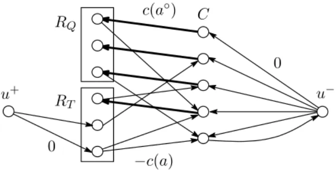
For the LM-polynomial matrixA(s) defined by (2),G(A) = (RQ∪RT, C;E(A)) has a matching M0 ={(i, i)|i∈RQ}, which corresponds to sd1, . . . , sdm. By applying augmenting path type algorithms to M0, we find a maximum weight matchingM with∂M ⊇RQ and |M|=mQ+k inG(A). Then, we construct an optimal solution (p, q, t) of DLP(A, k) fromM as follows.
Consider an auxiliary graph ˇGM = ( ˇV ,E) withˇ
Vˇ =RQ∪RT ∪C∪ {u+} ∪ {u−} and Eˇ =Ec∪M◦∪W+∪W−, whereu+ and u− are new vertices and
Ec={(i, j)|(i, j)∈E(A)} (copy ofE(A)), M◦ ={a◦|a∈M},
W+ ={(u+, i)|i∈RT \∂M},
W− ={(j, u−)|j ∈C\∂M} ∪ {(u−, j)|j∈C}.
We define the arc length γ : ˇE →Z by
γ(a) =
−c(a) (a∈Ec) c(a◦) (a∈M◦) 0 (a∈W+∪W−)
.
Let φ(i) be a shortest distance from u+ to i∈Vˇ with respect to the arc lengthγ in ˇGM. If there exists no path from u+ toi, then we putφ(i) =∞. We define
pi =φ(i) (∀i∈RQ∪RT), qj =φ(u−)−φ(j) (∀j∈C), t=−φ(u−). (4) Then (p, q, t) is an optimal dual solution of DLP(A, k) as follows.
0
u+ u−
−c(a) c(a◦) RQ
0 RT
C
Figure 2: An auxiliary graph ˇG= ( ˇV ,E), where heavy lines show edges in a matching.ˇ
Lemma 3.1. LetM be a maximum weight matching with ∂M ⊇ RQ and |M| =mQ+k in G(A). We define (p, q, t) by the auxiliary graph ˇGM and (4). Then (p, q, t) is an optimal dual solution of DLP(A, k). Moreover, if a weight function c is integer valued, then (p, q, t) is an integral solution.
Proof. Let us assume that there exists a shortest path P from u+ to i ∈ RT with negative distance. Then, the matching ˆM =M\{a∈M |a◦ ∈P∩M◦}∪(P∩Ec) satisfiesc( ˆM)> c(M), which contradicts the optimality ofM. Hence we have φ(i) ≥0 for each i∈RT. This implies the second constraint in DLP(A, k). Moreover, it holds that
φ(i) = 0 (∀i∈RT \∂M), (5)
because there exists an arc (u+, i) for each i∈RT \∂M.
Since there exists an arc (u−, j) for eachj ∈C, we have φ(j) ≤φ(u−), which implies the third constraint in DLP(A, k). Similarly, we obtainφ(j)≤φ(i)−c(e) for eache= (i, j)∈E(A).
Hence the first constraint in DLP(A, k) holds by (4).
Finally, we check the optimality of (p, q, t). There exist both arcs (i, j) and (j, i) for any (i, j) satisfying i=u− andj ∈C\∂M and (i, j)∈M. Hence we have
φ(j) =φ(u−) (∀j∈C\∂M), (6)
φ(j) =φ(i)−c(e) (∀e= (i, j)∈M). (7) It follows from (4)–(6) that
∑
i∈R
pi+∑
j∈C
qj+ (mQ+k)t=∑
i∈R
φ(i) +∑
j∈C
(φ(u−)−φ(j))−(mQ+k)φ(u−)
= ∑
i∈R∩∂M
φ(i) + ∑
j∈C∩∂M
(φ(u−)−φ(j))−(mQ+k)φ(u−)
= ∑
(i,j)∈M
(φ(i)−φ(j)) +|C∩∂M|φ(u−)−(mQ+k)φ(u−)
=c(M),
where the last step is due to (7) and |C∩∂M|=|M|=mQ+k. Thus we obtain
∑
i∈R
pi+∑
j∈C
qj+ (mQ+k)t=c(M),
which implies that (p, q, t) is optimal.
If a weight function c is integer valued, (p, q, t) is integral by the construction rule.
3.3 Test for Tightness
We describe a necessary and sufficient condition for ˆδLMk (A) =δLMk (A). For an integral feasible solution (p, q, t) of DLP(A, k), let us put
I∗ =RQ∪ {i∈RT |pi >0} and J∗ ={j∈C|qj >0}.
We call I∗ and J∗ active rows and active columns, respectively. The tight coefficient matrix A∗ = (A∗ij) is defined by
A∗ij = (the coefficient of spi+qj+t inAij(s)).
Note thatA∗ is an LM-matrix and A(s) = (Aij(s)) is expressed by
Aij(s) =spi+qj+t(A∗ij +A∞ij(s)) (8) with a strictly proper matrix A∞(s) = (A∞ij(s)).
The following lemma gives a necessary and sufficient condition for ˆδkLM(A) =δkLM(A), which is immediately derived from [18, Theorem 7].
Lemma 3.2. Let (p, q, t) be an optimal dual solution, I∗ and J∗ the active rows and columns, andA∗ the tight coefficient matrix. Then the following three conditions (a)–(c) are equivalent.
(a) δˆkLM(A) =δkLM(A) holds.
(b) There exists I ⊇I∗ and J ⊇J∗ such that rankA∗[I, J] =|I|=|J|=mQ+k.
(c) The following four conditions are satisfied:
(r1) rankA∗[R, C]≥mQ+k, (r2) rankA∗[I∗, C] =|I∗|, (r3) rankA∗[R, J∗] =|J∗|,
(r4) rankA∗[I∗, J∗]≥ |I∗|+|J∗| −(mQ+k).
Lemma 3.2 implies that we can check ˆδLMk (A) =δLMk (A) efficiently by computing the ranks of four LM-matricesA∗[R, C],A∗[I∗, C],A∗[R, J∗], andA∗[I∗, J∗]. This can be done by solving the corresponding independent matching problems described in Section 2.4. The optimality condition for (p, q, t) is given by the following variant, which is also derived from [18].
Lemma 3.3. Let (p, q, t) be a dual feasible solution, I∗ and J∗ the active rows and columns, and A∗ the tight coefficient matrix. Then (p, q, t) is optimal if and only if the following four conditions are satisfied:
(t1) term-rankA∗[R, C]≥mQ+k, (t2) term-rankA∗[I∗, C] =|I∗|, (t3) term-rankA∗[R, J∗] =|J∗|,
(t4) term-rankA∗[I∗, J∗]≥ |I∗|+|J∗| −(mQ+k).
3.4 Matrix Modification
Let A(s) be an LM-Laurent polynomial matrix such that δkLM(A) <δˆLMk (A). We describe the rule of modifying A(s) into another LM-Laurent polynomial matrix ˜A(s). Since δkLM(A) <
δˆkLM(A), it follows from Lemma 3.2 that at least one of conditions (r1)–(r4) is violated. In the test for tightness in Phase 2, we transform the tight coefficient matrix A∗ = (Q∗
T∗
) into another LM-matrix ˜A∗ =(Q˜∗
T˜∗
) by applying Algorithm for the Rank of an LM-matrix described in Section 2.4. WhenAlgorithm for the Rank of an LM-matrixterminates, it finds a nonsingular constant matrixU such that (
Q˜∗ T˜∗
)
= (
U O O I
) ( Q∗ T∗
) .
Let (p, q, t) be an optimal solution of DLP(A, k). With the use of U and (p, q, t), we transformA(s) into another LM-Laurent polynomial matrix ˜A(s) defined by
A(s) = diag[s˜ p1, . . . , spm] (
U O O I
)
diag[s−p1, . . . , s−pm]A(s). (9) In order to show that δLMk (A) is invariant under the transformation given in (9), we make use of the following lemma, which is immediately derived from [18, Lemma 11].
Lemma 3.4. Let A(s) and ˜U(s) be rational function matrices, and ˜A(s) = ˜U(s)A(s). Then δkLM(A) = δkLM( ˜A) if ˜U[RQ, RT] = O, det ˜U[RQ, RQ] is nonzero constant, and ˜U[RT, RT] is biproper.
The following lemma asserts δkLM(A) =δkLM( ˜A).
Lemma 3.5. Let A(s) be an LM-Laurent polynomial matrix and ˜A(s) the LM-Laurent poly- nomial matrix defined by (9). Then we haveδLMk (A) =δLMk ( ˜A).
Proof. For ˜U(s) = diag[sp1, . . . , spm] (
U O O I
)
diag[s−p1, . . . , s−pm], we denote the row/column sets by RQ∪RT. Then ˜U[RQ, RT] = O holds and ˜U[RT, RT] = I is biproper. In addition, det ˜U[RQ, RQ] = detU is nonzero constant, becauseU is a nonsingular constant matrix. Hence we obtainδkLM(A) =δkLM( ˜A) by Lemma 3.4.
Let ˜cij denote the degree of the (i, j) entry of ˜A(s). We now prove that an optimal solution (p, q, t) of DLP(A, k) is feasible for DLP( ˜A, k) but not optimal.
Lemma 3.6. Let A(s) be an LM-Laurent polynomial matrix with δkLM(A) < δˆkLM(A), and A(s) the LM-Laurent polynomial matrix defined by (9). Then an optimal solution (p, q, t) of˜ DLP(A, k) is feasible for DLP( ˜A, k) but not optimal.
Proof. We put
F(s) =s−tdiag[s−p1, . . . , s−pm] ˜A(s) diag[s−q1, . . . , s−qn].
The degree of the (i, j) entry of F(s) satisfies degFij(s) = ˜cij −pi−qj−t. By (8) and (9), F(s) is transformed as
F(s) =s−t (
U O O I
)
diag[s−p1, . . . , s−pm]A(s) diag[s−q1, . . . , s−qn]
= (
U O O I
)
(A∗+A∞(s)),
where A∞(s) denotes a strictly proper matrix. This indicates degFij(s) ≤ 0, because U and A∗ are constant matrices. Thus we obtain ˜cij −pi−qj −t ≤0, which implies that (p, q, t) is feasible for DLP( ˜A, k).
We show that (p, q, t) is not optimal for DLP( ˜A, k). Let us set ˜A∗(p,q,t) = (
U O O I
)
A∗. Then A˜∗(p,q,t) is the tight coefficient matrix of ˜A(s) with respect to (p, q, t). ByδLMk (A)<δˆLMk (A) and Lemma 3.2, at least one of conditions (r1)–(r4) is not fulfilled. Let us assume that A∗ violates (r2) and ˜A∗(p,q,t) is obtained by applying Algorithm for the Rank of an LM-matrix to A∗[I∗, C].
Then it follows from Lemma 2.3 that rank ˜A∗(p,q,t)[I∗, C] = term-rank ˜A∗(p,q,t)[I∗, C]. Hence we have
term-rank ˜A∗(p,q,t)[I∗, C] = rank ˜A∗(p,q,t)[I∗, C] = rankA∗[I∗, C]<|I∗|.
Thus ˜A∗(p,q,t)violates (t2), which implies that (p, q, t) is not optimal for DLP( ˜A, k) by Lemma 3.3.
If (r1), (r3), or (r4) is violated, we can prove that (p, q, t) is not optimal for DLP( ˜A, k) in a similar way.
3.5 Dual Updates
Let (p, q, t) be an optimal solution of DLP(A, k). By Lemma 3.6, (p, q, t) is feasible for DLP( ˜A, k). For (p, q, t) and another feasible solution (p′, q′, t′) of DLP( ˜A, k), we consider the amount of change ∆ in the value of the dual objective function defined by
∆ =
∑
i∈R
p′i+∑
j∈C
q′j+ (mQ+k)t′
−
∑
i∈R
pi+∑
j∈C
qj+ (mQ+k)t
.
With the use of (p, q, t), we construct a feasible solution (p′, q′, t′) which satisfies ∆ < 0. By repeating this procedure, we find an optimal dual solution of DLP( ˜A, k).
Let G∗ = (R, C;E∗) be a bipartite graph with E∗ = {(i, j) ∈ E( ˜A) | pi +qj +t = ˜cij}. Since (p, q, t) is not optimal for DLP( ˜A, k) by Lemma 3.6, at least one of conditions (t1)–(t4) for ˜A∗(p,q,t) is violated. For each case, we construct another feasible solution (p′, q′, t′) with
∆<0 as follows.
Case1: (t1) is violated
Since the maximum size of a matching inG∗= (R, C;E∗) is strictly less thanmQ+k,G∗ has a coverW with|W|< mQ+k. We now define
p′i =
{pi+ 1 (i∈R∩W)
pi (i∈R\W) , q′j =
{qj + 1 (j∈C∩W)
qj (j∈C\W) , t′ =t−1.
Then it holds that
∆ =|R∩W|+|C∩W| −(mQ+k) =|W| −(mQ+k)<0.
We show that (p′, q′, t′) is feasible for DLP( ˜A, k). First, consider an edge (i, j) ∈ E( ˜A) satisfying i ∈ W or j ∈ W. Since we have (p′i +qj′ +t′)−(pi +qj +t) ≥ 0, it holds that p′i+q′j+t′ ≥pi+qj+t≥˜cij by the feasibility of (p, q, t) for DLP( ˜A, k). Next, consider an edge (i, j) ∈ E( ˜A) satisfying i /∈ W and j /∈W. It follows from (i, j) ∈/ E∗ that pi+qj +t > ˜cij. Hence p′i+qj′ +t′=pi+qj +t−1>˜cij−1 holds. Thus, (p′, q′, t′) is feasible for DLP( ˜A, k).
Case2: (t2) is violated
Since the maximum size of a matching in G∗[I∗∪C] = (I∗, C;E∗[I∗∪C]) is strictly less than
|I∗|,G∗[I∗, C] has a coverW ⊆I∗∪C with|W|<|I∗|. We now define
p′i =
{pi (i∈(I∗∩W)∪(R\I∗))
pi−1 (i∈I∗\W) , q′j =
{qj+ 1 (j∈C∩W)
qj (j∈C\W) , t′ =t.
Then it holds that
∆ =−|I∗\W|+|C∩W|=|W| − |I∗|<0.
We can show that (p′, q′, t′) is feasible for DLP( ˜A, k) in a similar way to Case 1.
Case3: (t3) is violated
Since the maximum size of a matching inG∗[R∪J∗] = (R, J∗;E∗[R∪J∗]) is strictly less than
|J∗|,G∗[R, J∗] has a coverW ⊆R∪J∗ with|W|<|J∗|. We now define
p′i=
{pi+ 1 (i∈R∩W)
pi (i∈R\W) , qj′ =
{qj (j∈(J∗∩W)∪(C\J∗))
qj−1 (j∈J∗\W) , t′ =t.
Then it holds that
∆ =|R∩W| − |J∗\W|=|W| − |J∗|<0.
We can show that (p′, q′, t′) is feasible for DLP( ˜A, k) in a similar way to Case 1.
Case4: (t4) is violated
Since the maximum size of a matching inG∗[I∗∪J∗] = (I∗, J∗;E∗[I∗∪J∗]) is strictly less than
|I∗|+|J∗| −(mQ+k),G∗[I∗, J∗] has a coverW ⊆I∗∪J∗ with|W|<|I∗|+|J∗| −(mQ+k).
We now define p′i =
{pi−1 (i∈I∗\W)
pi (i∈(I∗∩W)∪(R\I∗)), q′j =
{qj−1 (j∈J∗\W)
qj (j∈(J∗∩W)∪(C\J∗)), t′=t+ 1.
Then it holds that
∆ =−|I∗\W| − |J∗\W|+ (mQ+k) =|W| −(|I∗|+|J∗| −(mQ+k))<0.
We can show that (p′, q′, t′) is feasible for DLP( ˜A, k) in a similar way to Case 1.
4 Complexity Analysis
This section is devoted to complexity analysis of our combinatorial relaxation algorithm.
4.1 Worst Case Analysis
We analyze the complexity of our combinatorial relaxation algorithm, which is now described as follows.
Algorithm for Computing δLMk (A)
Step 1 Find a maximum weight matching M in G(A) by using an efficient combinatorial algorithm.
Step 2 Construct an optimal solution (p, q, t) of DLP(A, k) from M.
Step 3 Apply Algorithm for the Rank of an LM-matrix to A∗[R, C], A∗[I∗, C], A∗[R, J∗], and A∗[I∗, J∗]. If (r1)–(r4) hold, then return ˆδkLM(A) and halt.
Step 4 ModifyA(s) to another matrix ˜A(s) defined by (9).
Step 5 Construct an optimal solution (˜p,q,˜ ˜t) of DLP( ˜A, k) by performing the procedure given in Section 3.5. Go back to Step 3.
This algorithm is dominated by the computation of ˜A(s) in Step 4. We discuss its time and space complexities in the following.
For an integral optimal solution (p, q, t) of DLP(A, k), we denote diag[sp1, . . . , spm] and diag[sq1, . . . , sqn] by Vr(s) and Vc(s), respectively. By the definition of the tight coefficient matrixA∗, the LM-Laurent polynomial matrixA(s) is expressed as
A(s) =stVr(s) (
A∗+1
sA1+ 1
s2A2+· · ·+ 1 slAl
) Vc(s)