Uptake and Storage of Carbon Dioxide in the Ocean:
The Global C02 Survey
Richard A. Feely
Pacific Marine and Environmental Laboratory
National Oceanic and Atmospheric Administration • Seattle, Washington USA Christopher L. Sabine
University of Washington • Seattle, Washington USA Taro Takahashi
Lamont-Doherty Earth Observatory. Palisades, New York USA Rik Wanninkhof
Atlantic Oceanographic and Meteorological Laboratory
National Oceanic and Atmospheric Administration. Miami, Florida USA
Introduction
Human activity is rapidly changing the composi- tion of the earth's atmosphere, contributing to warm- ing from excess carbon dioxide (CO2) along with other trace gases such as water vapor, chlorofluorocarbons, methane and nitrous oxide. These anthropogenic
"greenhouse gases" play a critical role in controlling the earth's climate because they increase the infrared opacity of the atmosphere, causing the surface of the planet to warm. The release of CO2 from fossil fuel con- sumption or the burning of forests for farming or pas- hare contributes approximately 7 petagrams of carbon (1 Pg C = 1 x 10 '5 g C) to the atmosphere each year.
Approximately 3 Pg C of this "anthropogenic COd' accumulates in the atmosphere annually, and the remaining 4 Pg C is stored in the terrestrial biosphere and the ocean.
Where and how land and ocean regions vary in their uptake of CO2 from year to year is the subject of much scientific research and debate. Future decisions on regulating emissions of greenhouse gases should be based on more accurate models of the global cycling of carbon and the regional sources and sinks for anthro- pogenic CO2, models that have been adequately tested against a well-designed system of measurements. The construction of a believable present-day carbon budget is essential for the reliable prediction of changes in atmospheric CO2 and global temperatures from avail- able emissions scenarios.
The ocean plays a critical role in the global carbon cycle as a vast reservoir that exchanges carbon rapidly with the atmosphere, and takes up a substantial por- tion of anthropogenically-released carbon from the
atmosphere. A significant impetus for carbon cycle research over the past several decades has been to achieve a better understanding of the ocean's role as a sink for anthropogenic CO2. There are only three global reservoirs with exchange rates fast enough to vary sig- nificantly on the scale of decades to centuries: the atmosphere, the terrestrial biosphere and the ocean.
Approximately 93% of the carbon is located in the ocean, which is able to hold much more carbon than the other reservoirs because most of the CO2 that diffuses into the oceans reacts with seawater to form carbonic acid and its dissociation products, bicarbonate and car- bonate ions (Figure 1).
Our present understanding of the temporal and spatial distribution of net CO2 flux into or out of the ocean is derived from a combination of field data, which is limited by sparse temporal and spatial cover- age, and model results, which are validated by com- parisons with the observed distributions of tracers, including natural carbon-14 (14C), and anthropogenic chlorofluorocarbons, tritium (3H) and bomb 14C. The lat- ter two radioactive tracers were introduced into the atmosphere-ocean system by atomic testing in the mid 20 ~ century. With additional data from the recent glob- al survey of CO2 in the ocean (1991-1998), carried out cooperatively as part of the Joint Global Ocean Flux Study (JGOFS) and the World Ocean Circulation Experiment (WOCE) Hydrographic Program, it is now possible to characterize in a quantitative way the regional uptake and release of CO2 and its transport in the ocean. In this paper, we summarize our present understanding of the exchange of CO2 across the air-sea Oceanography • VoL 14 • No. 4/2001
18
Atmosphere
CO2(g ) 1XCO2 2XCO 2
Gas E c hange 280
CO2(aq)+ H20 ~ H2CO 3 8 Carbonic acid
H2CO3 H++HCO3" 1617
Bicarbonate
HCO3" ~ H++CO32- 268 Carbonate
1893
R1;
560
15 1850
176 2040 DIC
7 CJl nH
Surface ocean
Figure 1. Schematic diagram of the carbon dioxide (C02) system in seawater. The 1 x C02 concentrations are for a surface ocean in equilibrium with a pre-industrial atmospheric C02 level of 280 ppm. The 2 x C02 concentrations are for a surface ocean in equilibrium with an atmospheric C02 level of 560 ppm. Current model projections indicate that this level could be reached sometime in the second half of this century. The atmospheric values are in units of ppm. The oceanic concentrations, which are for the surface mixed layer, are in units of #mol kg -1.
interface and the storage of natural and anthropogenic CO2 in the ocean's interior.
Background
The history of large-scale CO2 observations in the ocean date back to the 1970s and 1980s. Measurements of the partial pressure of CO2 (pCO~), total dissolved inorganic carbon (DIC) and total alkalinity (AT) were m a d e during the global Geochemical Ocean Sections (GEOSECS) expeditions between 1972 and 1978, the Transient Tracers in the Oceans (TTO) N o r t h Atlantic and Tropical Atlantic Surveys in 1981-83, the South Atlantic Ventilation Experiment (SAME) from 1988-1989, the French Southwest Indian Ocean experiment, and n u m e r o u s other smaller expeditions in the Pacific and Indian Oceans in the 1980s. These studies p r o v i d e d marine chemists with their first view of the carbon sys- tem in the global ocean.
These data were collected at a time w h e n no com- m o n reference materials or standards were available. As a result, analytical differences between measurement groups were as large as 29 ~lrnol kg -1 for both DIC and Av which corresponds to more than 1% of the ambient values. Large adjustments h a d to be m a d e for each of the data sets based on deepwater comparisons at near- b y stations before individual cruise data could be com- pared. These differences were often nearly as large as the anthropogenic CO2 signal that investigators were trying to determine (Gruber et al., 1996). Nevertheless, these early data sets m a d e u p a c o m p o n e n t of the sur- face ocean pCO2 measurements for a global climatology and also p r o v i d e d researchers with n e w insights into the distribution of anthropogenic CO2 in the ocean, par- ticularly in the Atlantic Ocean.
At the onset of the Global Survey of CO2 in the Ocean (Figure 2), several events took place in the United Oceanography " Vol. 14 • No. 4/2001
19
40E 80E 120E 160E 160W 120W 80W 4 0 W 0 °
4(
0 o 0 o
4(
40E 80E 120E 160E 1 6 0 W 1 2 0 W 80W 4 0 W 0 °
Figure 2. The Global Survey of C02 in the Ocean: cruise tracks and stations occupied between 1991 and 1998.
States and in international CO2 measurement communi- ties that significantly improved the overall precision and accuracy of the large-scale measurements. In the United States, the CO2 measurement program was co-funded by the Department of Energy (DOE), the National Oceanic and Atmospheric Administration (NOAA) and the National Science Foundation (NSF) under the tech- nical guidance of the U.S. CO2 Survey Science Team.
This group of academic and government scientists adopted and perfected the recently developed coulo- metric titration method for DIC determination that had demonstrated the capability to meet the required goals for precision and accuracy. They advocated the develop- ment and distribution of certified reference materials (CRMs) for DIC, and later for A~, for international dis- tribution under the direction of Andrew Dickson of Scripps Institution of Oceanography (see sidebar). They also supported a shore-based intercomparison experi- ment under the direction of Charles Keeling, also of Scripps. Through international efforts, the development of protocols for CO2 analyses were adopted for the CO2 survey. The international partnerships fostered by JGOFS resulted in several intercomparison CO2 exercis- es hosted by France, Japan, Germany and the United States. Through these and other international collabora- tive programs, the measurement quality of the CO2 sur- vey data was well within the measurement goals of _+ 3
~mol kg -1 and + 5 ~rnol kg -1, respectively, for DIC and AT.
Several other developments significantly enhanced the quality of the CO2 data sets during this period. New methods were developed for automated underway and
discrete pCO2 measurements. An extremely precise method for pH measurements based on spectrophotom- etry was also developed by Robert Byrne and his col- leagues at the University of South Florida. These improvements ensured that the internal consistency of the carbonate system in seawater could be tested in the field whenever more than two components of the car- bonate system were measured at the same location and time. This allowed several investigators to test the over- all quality of the global CO2 data set based upon CO2 sys- tem thermodynamics. Laboratories all around the world contributed to a very large and internally consistent glob- al ocean CO2 data set determined at roughly 100,000 sam- ple locations in the Atlantic, Pacific, Indian and Southern oceans (Figure 2). The data from the CO2 survey are avail- able through the Carbon Dioxide Information and Analysis Center (CDIAC) at Oak Ridge National Laboratory as Numeric Data Packages and on the World Wide Web (http://cdiac.esd.ornl.gov/home.html). Taro Takahashi and his collaborators have also amassed a large database of surface ocean pCO2 measurements, spanning more than 30 years, into a pCO2 climatology for the global ocean (Takahashi et al., in press). These data have been used to determine the global and regional flux- es for CO2 in the ocean.
C02 Exchange Across the Air-Sea Interface
In seawater, CO2 molecules are present in three major forms: the undissociated species in water, [CO2]aq, and two ionic species, [HCO3-] and [COd-]
(Figure 1). The concentration of [CO~]aq depends upon
Oceanography • Vol. 14 • No. 4/2001
2O
Andrew G. Dickson
Scripps Institution of Oceanography Universily of California, San Diego, La Jolla California USA
High-quality measurements of carbon dioxide (CO2) in the ocean have been an integral part of JGOFS. Despite their importance for understanding the oceanic carbon cycle, measurements made by different groups were rarely comparable in the past. A signifi- cant contribution of U.S. JGOFS has been to produce and distribute reference materi- als for oceanic CO2 measurements. These materials are stable substances for which one or more properties are established sufficiently well to calibrate a chemical analyzer or to validate a measurement process.
Our laboratory at Scripps Institution of Oceanography (SIO), established in ! 989 with U.S. JGOFS support from the National Science Foundation (NSF), has prepared over 50 separate batches of reference material and has distributed more than 25,000 bot- tles of this material to scientists in 33 laboratories in the U.S. and 58 facilities in 24 other countries. The reference materials have been used both as a basis for collabora~
tive studies and as a means of quality control for at-sea measurements. Although most JGOFS field studies are over, we are still distributing more than 2,000 bottles per year
and demand is again growing.
To prepare the reference material, we sterilize a batch of seawater, equilibrate it to a virtually constant partial pressure of CO2 and deliver it for bottling. For each batch, sur- face seawater collected on ships of opportunity and stored in our laboratory is pumped into a holding tank using filters and a sterilizing unit to reduce contamination. When the holding tank is nearly full, mercuric chloride is added as a biocide. The seawater is then recirculated for a few days to ensure complete mixing and enable some gas exchange with filtered air that is pumped through the head-space of the tank. Finally, aliquots of the seawater are pumped through an ultraviolet sterilizing unit and a O. 1 tsm filter and into clean 500-mL glass bottles. These are sealed with grease and labeled.
Random samples from each batch of reference material are analyzed over a period of 2-3 months for both total dissolved inorganic carbon (G) and total alkalinity (AT), and the results are used to certify the batch before it is distributed. From the start, we used a high-quality method for the determination of CT in which a weighed amount of sea- water is acidified and the CO2 extracted under vacuum, purified and determined mano- metrically. These analyses are carried out in
the laboratory of C.D. Keeling at SIO using equipment originally developed for the cali- bration of gases for atmospheric CO2 meas- urements.
By 1996, we had also developed an accurate method for the measurement of AT using a two-stage potentiometric, open-cell titration with coulometrically analyzed hydrochloric acid. Once this latter method was being employed routinely to certify new batches of reference material, we used it retrospectively to analyze archived samples from earlier batches.
The uncertainties of these analyses used for certification are + 1.5 pmol kg ~ in CT and + 2 mol pkg ~ in A., and our reference materials have been shown to be stable for more than 3 years. We are now working on providing pH values on future reference materials, as well as values for 6~3C.
As part of U.S. JGOFS, the Department of Energy (DOE) supported measurements of
!1
21
ocean CO2 system parameters on sections of the WOCE Hydrographic Programme one-time survey. The CO2 Survey Science Team adopted the use of our reference materials as soon as they were available in early 1991 and continued to use them on subsequent cruises. Measurements made on reference materials while at sea were used to ascertain data quality on these expeditions and are thought to have contributed substantially to the overall high quality of the resultant data set.
A further indication that the use of reference materials has improved oceanographic data quality can be seen by examining the degree of agreement between measurements for deep water masses obtained where two separate cruises intersect. For cruises where reference materials were available, measurements of CT in deep water now typically agree to within 2 pmol kgL This is in sharp con- trast to the problems encountered over the years with earlier ocean carbon data sets, where adjustments of as much as 15-20 pmol kg ~ were fairly common. The high-quality data sets now available provide a resource for synthesis and modeling that makes it pos- sible to put together a coherent global view of the oceanic carbon cycle.
Acknowledgements
This work was supported by NSF through grants OCE8800474, OCE9207265, OCE9521976 and OCE-9819007 and by DOE through Pacific Northwest National Laboratory subcontract No. 121945 and grant DEFG0392ER61410. This work was encouraged early on by Neil Andersen, then at NSF, and has benefited from advice from C.D. Keeling, the members of the DOE CO2 Survey Science Team and colleagues from the National Oceanic and Atmospheric Administration. I should also like to thank Justine Afghan and George Anderson, who carried out most of the technical work involved in this project, as well as Guy Emanuele and Peter Guenther from the Carbon Dioxide Research Group at SIO, who performed the CT analyses.
the temperature and chemical composition of seawater.
The amount of [CO2]aq is proportional to the partial pressure of CO2 exerted by seawater. The difference between the pCO2 in surface seawater and that in the overlying air represents the thermodynamic driving potential for the CO2 transfer across the sea surface.
The pCO2 in surface seawater is known to vary geo- graphically and seasonally over a range between about 150/,latin and 750 ~atm, or about 60% below and 100%
above the current atmospheric pCO2 level of about 370 /satm. Since the variation of pCO2 in the surface ocean is much greater than the atmospheric pCO2 seasonal variability of about 20/Jatm in remote uncontaminated marine air, the direction and magnitude of the sea-air CO2 transfer flux are regulated primarily by changes in the oceanic pCO2. The average pCO= of the global ocean is about 7/~atm lower than the atmosphere, which is the primary driving force for uptake by the ocean (see Figure 6 in Karl et al., this issue).
The pCO2 in mixed-layer waters that exchange CO2 directly with the atmosphere is affected primarily by temperature, DIC levels and AT. While the water tem- perature is regulated by physical processes, including solar energy input, sea-air heat exchanges and mixed- layer thickness, the DIC and A T are primarily con- trolled by the biological processes of photosynthesis and respiration and by upwelling of subsurface waters rich in respired CO= and nutrients. In a parcel of sea- water with constant chemical composition, pCO2 would increase by a factor of 4 when the water is warmed from polar temperatures of about -1.9 °C to equatorial temperatures of about 30 °C. On the other hand, the DIC in the surface ocean varies from an aver- age value of 2150 ~rnol kg -1 in polar regions to 1850
~rnol kg-' in the tropics as a result of biological process- es. This change should reduce pCO2 by a factor of 4. On
a global scale, therefore, the magnitude of the effect of biological drawdown on surface water pCO2 is similar in magnitude to the effect of temperature, but the two effects are often compensating. Accordingly; the distri- bution of pCO2 in surface waters in space and time, and therefore the oceanic uptake and release of CO=, is gov- erned by a balance between the changes in seawater temperature, net biological utilization of CO2 and the upwelling flux of subsurface waters rich in CO2.
Database and Methods
Surface-water pCO2 has been determined with a high precision (+_2/Jatm) using underway equilibrator- CO2 analyzer systems over the global ocean since the International Geophysical Year of 1956-59. As a result of recent major oceanographic programs, including the global CO2 survey and other international field studies, the database for surface-water pCO2 observations has been improved to about 1 million measurements with several million accompanying measurements of SST, salinity and other necessary parameters such as baro- metric pressure and atmospheric CO2 concentrations.
Based upon these observations, a global, monthly cli- matological distribution of surface-water pCO2 in the ocean was created for a reference year 1995, chosen because it was the median year of pCO2 observations in the database. The database and the computational method used for interpolation of the data in space and time will be briefly described below.
For the construction of climatological distribution maps, observations made in different years need to be corrected to a single reference year (1995), based on sev- eral assumptions explained below (see also Takahashi et al., in press). Surface waters in the subtropical gyres mix vertically at slow rates with subsurface waters because of strong stratification at the base of the mixed Oceanography • VoL 14 • No. 4/2001
22
layer. As a result, they are in contact with the atmosphere and can exchange COs for a long time. Consequently, the pCO2 in these warm waters follows the increasing trend of atmospheric CO2 concentrations, as observed by Inoue et al. (1995) in the western North Pacific, by Feely et al.
(1999) in the equatorial Pacific and by Bates (2001) near Bermuda in the western North Atlantic. Accordingly, the pCO2 measured in a given month and year is corrected to the same month in the reference year 1995 using the fol- lowing atmospheric COs concentration data for the plan- etary boundary layer: the GLOBALVIEW-CO2 database (2000) for observations made after 1979 and the Mauna Loa data of Keeling and Whorf (2000) for observations before 1979 (reported in CDIAC NDP-001, revision 7).
In contrast to the waters of the subtropical gyres, sur- face waters in high-latitude regions are mixed convec- tively with deep waters during fall and winter, and their CO2 properties tend to remain unchanged from year to year. They reflect those of the deep waters, in which the effect of increased atmospheric COs over the time span of the observations is diluted to undetectable levels (Takahashi et al., in press). Thus no correction is neces- sary for the year of measurements.
Distribution Maps for Climatological Mean Sea-air pC02 Difference
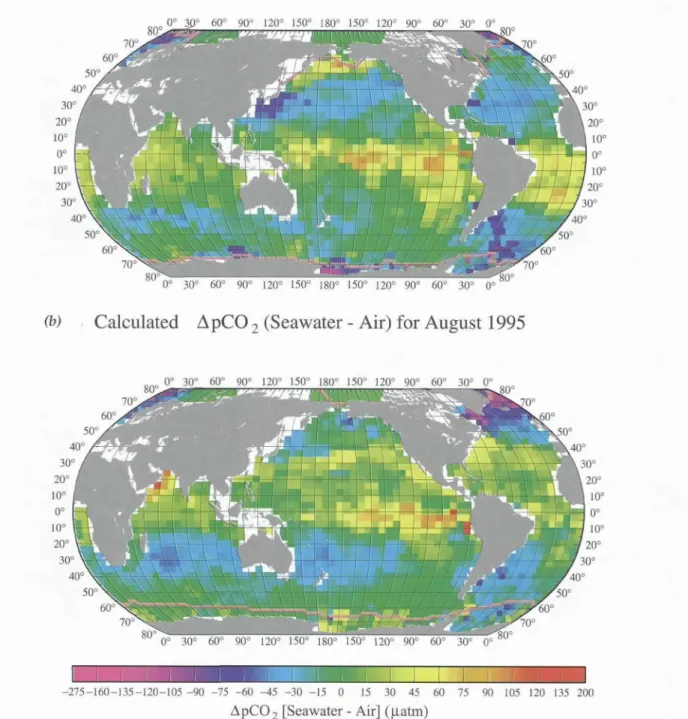
Figure 3 shows the distribution of climatological mean sea-air pCO2 difference (ApCO2) during February (Figure 3a) and August (Figure 3b) for the reference year 1995. The yellow-red colors indicate oceanic areas where there is a net release of COs to the atmosphere, and the blue-purple colors indicate regions where there is a net uptake of CO2. The equatorial Pacific is a strong source of CO2 to the atmosphere throughout the year as a result of the upwelling and vertical mixing of deep waters in the central and eastern regions of the equatorial zone. The intensity of the oceanic release of CO2 decreases west- ward in spite of warmer temperatures to the west. High levels of COs are released in parts of the northwestern subarctic Pacific during the northern winter and the Arabian Sea in the Indian Ocean during August. Strong convective mixing that brings up deep waters rich in COs produces the net release of COs in the subarctic Pacific.
The effect of increased DIC concentration surpasses the cooling effect on pCO2 in seawater during winter. The high pCO2 in the Arabian Sea water is a result of strong upwelling in response to the southwest monsoon. High pCO2 values in these areas are reduced by the intense primary production that follows the periods of upwelllng.
The temperate regions of the North Pacific and Atlantic oceans take up a moderate amount of COs (blue) during the northern winter (Figure 3a) and release a moderate amount (yellow-green) during the northern summer (Figure 3b). This pattern is the result primarily of seasonal temperature changes. Similar seasonal changes are observed in the southern temperate oceans.
Intense regions of CO2 uptake (blue-purple) are seen in the high-latitude northern ocean in summer (Figure 3b)
and in the high-latitude South Atlantic and Southern oceans near Antarctica in austral summer (Figure 3a).
The uptake is linked to high biological utilization of CO2 in thin mixed layers. As the seasons progress, ver- tical mixing of deep waters eliminates the uptake of COs.
These observations point out that the Z~CO2 in high-latitude oceans is governed primarily by deep- water upwelling in winter and biological uptake in spring and summer, whereas in the temperate and sub- tropical oceans, the ApCO2 is governed primarily by water temperature. The seawater ApCO2 is highest dur- ing winter in subpolar and polar waters, whereas it is highest during summer in the temperate regions. Thus the seasonal variation of ApCO2 and therefore the shift between net uptake and release of CO2 in subpolar and polar regions is about 6 months out of phase with that in the temperate regions.
The ApCO2 maps are combined with the solubility (s) in seawater and the kinetic forcing function, the gas transfer velocity (k), to produce the flux:
F = k , s . A p C 0 2 (1)
The gas transfer velocity is controlled by near-sur- face turbulence in the liquid b o u n d a r y layer.
Laboratory studies in wind-wave tanks have shown that k is a strong but non-unique function of wind speed. The results from various wind-wave tank inves- tigations and field studies indicate that factors such as fetch, wave direction, atmospheric boundary layer sta- bility and bubble entrainment influence the rate of gas transfer. Also, surfactants can inhibit gas exchange through their damping effect on waves. Since effects other than wind speed have not been well quantified, the processes controlling gas transfer have been para- meterized solely with wind speed, in large part because k is strongly dependent on wind, and global and regional wind-speed data are readily available.
Several of the frequently used relationships for the estimation of gas transfer velocity as a function of wind speed are shown in Figure 4 to illustrate their different dependencies. For the Liss and Merlivat (1986) rela- tionship, the slope and intercept of the lower segment was determined from an analytical solution of transfer across a smooth boundary. For the intermediate wind regime, the middle segment was obtained from a field study in a small lake, and results from a wind-wave tank study were used for the high wind regime after applying some adjustments. This relationship is often considered the lower bound of gas transfer-wind speed relationships.
The quadratic relationship of Wanninkhof (1992) was constructed to follow the general shape of curves derived in wind-wave tanks but adjusted so that the global mean transfer velocity corresponds with the long-term global average gas transfer velocity deter- mined from the invasion of bomb 14C into the ocean.
Because the bomb 1~C is also used as a diagnostic or tun- Oceanography • VoL 14 • No. 4/2001
23
(a) Calculated ApCO 2 (Seawater - Air) for February 1995
3 0 2 0 ° 1 0 o
0 o 1 0 ° 2 0 °
3 0
0 o 3 0 ° 6 0 ° 9 0 ° 1 2 0 ° 1 5 0 ° 1 8 0 ° 1 5 0 ° 1 2 0 ° 9 0 ° 6 0 °
u v OO
(b) Calculated
3 0 ° 6 0 ° 9 0 ° 1 2 0 ° 1 5 0 ° 1 8 0 ° 1 3 U ° 1 2 0 ° 9 0 ° 6 0 ° 3 0 ° 0 o
3 0 ° 0 o
ApCO 2 (Seawater - Air) for August 1995
0 o 2 0 °
1 0 ° 0 o 1 0 ° 2 0 ° 0 o
0 o 3 0 ° 6 0 ° 9 0 ° 1 2 0 ° 1 5 0 ° 1 8 0 ° 1 5 0 ° 1 2 0 ° 9 0 o 6 0 ° g~o 0 o
U ~ 3 U ~ o u - '~u- I Z U - 1 3 u - l b t Y I D U - ~.d.U" Y U " O U - 3t) ~ U ~
~0 o 1 0 ° 0 o 1 0 o
~_0 0 )o
- 2 7 5 - 1 6 0 - 1 3 5 - 1 2 0 - 1 0 5 - 9 0 - 7 5 - 6 0 - 4 5 - 3 0 - 1 5 0 1 5 3 0 4 5 6 0 7 5 9 0 1 0 5 1 2 0 1 3 5 2 0 0
ApCO 2 [Seawater - Air] (gatm)
Figure 3. Distribution of climatologicaI mean sea-air pC02 difference (ApCO2) for the reference year 1995 representing non- El Niho conditions in February (a) and August (b). These maps are based on about 940,000 measurements of surface water pCOJrom 1958 through 2000. The pink lines indicate the edges of ice fields. The yellow-red colors indicate regions with a net release of C02 into the atmosphere, and the blue-purple colors indicate regions with a net uptake of COJrom the atmos- phere. The mean monthly atmospheric pC02 value in each pixel in 1995, (pCO2)air, is computed using (pCO2)air = (C02)air x (Pb -pH20). (C02)air is the monthly mean atmospheric C02 concentration (mole fraction of C02 in dry air)from the GLOBALVIEW database (2000); Pb is the climatological mean barometric pressure at sea level from the Atlas of Surface Marine Data (1994); and the water vapor pressure, pH20, is computed using the mixed layer water temperature and salin- ity from the World Ocean Database (1998) of NODC/NOAA. The sea-air pCO2 difference values in the reference year 1995 have been computed by subtracting the mean monthly atmospheric pC02 value from the mean monthly surface ocean water pC02 value in each pixeI.
Oceanography • VoL 14 • No. 4/2001
24
Table 1
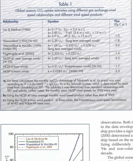
Global oceanic C02 uptake estimates using different gas exchange-wind speed relationships and different wind speed products a.
Relationship Liss & Merlivat [1986]
Equalion
k=0.17Um (U,o <3.6ms")
k= 2.85 Um- 9.65 (3.6 m s-'<U~o < 13 m s "1)
Flux {Pg c yr')
k= 5.9 U,0 - 49.3 (U,0 > 13 m s") -1.0 Wanninkhof [1992] [W-92] k= 0.39 U102 (long term averaged winds) -1.8 Wanninkhof & McGillis (1999) k= 1.09 U,0 - 0.333 Um 2 + 0.078 Um 3 -3.0
[W&M-99] (long term averaged winds)
Nightingale et al. [2000] k= 0.333 U10 + 0.222 U~02 -1.5 NCEP-41 year average winds b k= 0.39 U~02 (long term averaged winds) -2.2
[W-921
NCEP 6-hour winds c k= 0.31 U,02 (instantaneous winds) [W-92] -1.7
NCEP 6-hours winds ° k = 0.0283 U,03 [W&M-99] -2.3
a: For these calculations the monthly ApCO2 climatology of Takahashi et al. (in press) was used accordin¢l to: F = k (Sc/660) ~/2 s ~pCO2, Sc is the Schmldt number, which is determined for each pixel from climatoloqical SST. The solubility s was determined from standard relationships with SST and salinity. Un'fess noted, the monthly mean NCEP wind speeds for 1995 were used.
b: Using the NCEP 41-year average monthly wind speed product rather than that of 1995.
¢ : Using the NCEP &hour wind product. In these cases, the instantaneous wind speed formulations of W-92 and W&M-99 were used.
100
80
L 60
E o
,_~40
20
• • I • ' • I ' ' ' I ' ' " I • • • I • ' ' I ' ' ' I " ! '
... Liss & Merlivat-86 !
Wanninkhof-92 I ]
==,e,- Wanninkhof & McGillis-99 I [ I--" Nightingale et al" 2000 ~ [ ~ /
/ .-'.
0 2 4 6 8 10 12 14 16
Ulo [m s-l]
Figure 4. Graph of the different relationships that have been developed for the estimation of the gas transfer velocity, k, as a function of wind speed. The relationships were developed from wind-wave tank experiments, oceanic observations, global constraints and basic theo- ry. The different forms of the relationships are summa- rized in Table 1. U~o is wind speed at 10 m above the sea
surface.
ing parameter in global ocean biogeochemical circu- lation models, this parame- terization yields internally consistent results when used with these models, making it one of the more favored parameterizations.
Using the same long- term global 14C constraint but basing the general shape of the curve on recent CO2 flux observations over the North Atlantic determined using the covariance tech- nique, Wanninkhof and McGillis (1999) proposed a significantly stronger (cubic) dependence with wind speed. This relationship shows a weaker dependence on wind for wind speeds less than 10 ms -1 and a signifi- cantly stronger dependence at higher wind speeds.
However, the relationship is not well constrained at high wind speeds because of the large scatter in the scarce observations. Both the U 2 and U 3 relationships fit with- in the data envelope of the study, but the U 3 relation- ship provides a significantly better fit. Nightingale et al.
(2000) determined a gas exchange-wind speed relation- ship based on the results of a series of experiments uti- lizing deliberately injected sulfur hexafluoride (SF6), 3He and non-volatile tracers performed in the last decade.
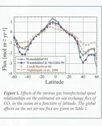
The global oceanic CO2 uptake using different wind speed/gas transfer velocity parameterizations differs by a factor of three (Table 1). The wide range of global CO2 fluxes for the different relationships illustrates the large range of results and assumptions that are used to produce these relationships. Aside from differences in global oceanic CO2 uptake, there are also significant regional differences. Figure 5 shows that the relation- ship of W&M-99 yields systematically lower evasion rates in the equatorial region and higher uptake rates at high latitudes compared with W-92, leading to signifi- cantly larger global CO2 uptake estimates.
In addition to the non-unique dependence of gas exchange on wind speed, which causes a large spread in global air-sea CO2 flux estimates, there are several other factors contributing to biases in the results.
Global wind-speed data obtained from shipboard observations, satellites and data assimilation tech- niques show significant differences on regional and global scales. Because of the non-linearity of the rela- tionships between gas exchange and wind speed, sig- nificant biases are introduced in methods of averaging Oceanography • Vol. 14 • No. 4/2001
25
] I dYeS
--, o £olP .
_, )
! ~ Wanninkhof-92
- - I t - - W a n n i n k h o f & McGillis-99
~3 • • o ' ' Liss&Merlivat-86 - - + - - Nightingale et al., 2000
- 4 i i i i , • , i . , , i , , , , , ,