ロボットマニピュレータの関節摩擦の同定，補償お よび推定

ロボットマニピュレータの関節摩擦の同定，補償お よび推定

岩谷, 正義

https://doi.org/10.15017/1807023

出版情報：Kyushu University, 2016, 博士（工学）, 課程博士 バージョン：

権利関係：Fulltext available.

by

Masayoshi Iwatani

Firstly, I would like to thank my supervisor, Dr. Ryo Kikuuwe, for his advices, instructions and patience. Without his devotion of huge amount of effort and time, writing my disserta- tion cannot be completed. Furthermore, his words have encouraged me and have provided me new viewpoints about research and work, which must help me to survive the future of life.

I also would like to sincerely thank Dr. Motoji Yamamoto for his support in my research work. His guidelines, advices and encouragements have helped my research work.

I also would like to thank Dr. Takahiro Kondou and Dr. Ryo Kurazume, who are the members of my dissertation supervisory committee, for their review and comments for this dissertation.

I wish to express my thanks to Dr. Svinin Mikhail, Dr. Kenji Tahara, Dr. Takeshi Ikeda and Dr. Yasutaka Nakashima for their suggestions and comments, which have been great support in academic and personal life.

I want to thank previous Ph.D. students of Control Engineering, Dr. Shanhai Jin, Dr. Xi- aogang Xiong and Dr. Aung Myo Than Sin for their advises and constructive discussions especially about friction, noise reduction filters and force control schemes.

Special thanks go to Mr. Kouki Shinya for his contributions in developing experimental setups we have used and in maintenance of laboratory’s safety and cleanliness.

Throughout my laboratory life, I have been helped by many laboratory members. I would like to thank Ms. Midori Tateyama, Ms. Ayako Kashiwagi and Ms. Mizuho Nagatomi for their kind help in various forms. I am also grateful to all previous and current student members, especially Dr. Yuki Matsutani, Dr. Aung Myo Thant Sin, Dr. Noriyasu Iwamoto, Dr. Akihiro Morinaga, Mr. Seunghyun Choi, Mr. Gyuho Byun, Mr. Masahiro Kadosaki,

I

Mr. Soichiro Kanda, Mr. Yang Bai, Mr. Yuuki Nozawa, Mr. Tomofumi Watari, who have been helpful and encouraging in my laboratory life.

Finally, I am deeply thankful to my family for their moral and financial support through-

out my Ph.D. research.

Acknowledgements I

List of figures VI

List of tables IX

1 Introduction 1

1.1 Joint Friction in Robotic Systems . . . . 1

1.2 Modeling of Friction . . . . 2

1.3 Identification of Joint Friction . . . . 5

1.3.1 Sliding region and presliding region . . . . 5

1.3.2 On-line method . . . . 6

1.4 Compensation of Joint Friction . . . . 7

1.4.1 Model-based compensation . . . . 7

1.4.2 Dither . . . . 8

1.5 Estimation of Joint Friction Force . . . . 9

1.5.1 External force estimation . . . . 9

1.5.2 Sensorless admittance control . . . . 11

1.6 Major Achievements . . . . 12

1.7 Organization . . . . 13

2 Identification of Joint Friction: Identification Procedure for Robotic Joints with Limited Motion Ranges 15 2.1 Introduction . . . . 15

2.2 Related Work . . . . 16

III

2.3 Procedure . . . . 17

2.3.1 Overview . . . . 17

2.3.2 Details . . . . 18

2.3.3 Analysis on the influence of inertia and gravity . . . . 23

2.4 Experiment: Identification . . . . 24

2.4.1 Experimental setup . . . . 24

2.4.2 Sensitivity to the choice of A . . . . 26

2.4.3 Sensitivity to the posture . . . . 29

2.5 Experiment: Friction Compensation . . . . 31

2.5.1 Manual moving . . . . 33

2.5.2 Feedback position tracking . . . . 36

2.6 Summary . . . . 38

3 Compensation of Joint Friction: New Elastoplastic Friction Compensator 40 3.1 Introduction . . . . 40

3.2 Experimental Setup . . . . 42

3.2.1 Overview . . . . 42

3.2.2 Presliding behavior . . . . 43

3.2.3 Rate-dependent friction . . . . 44

3.3 Conventional Elastoplastic Friction Model . . . . 46

3.3.1 Details . . . . 46

3.3.2 Problem in the application to friction compensation . . . . 48

3.4 Proposed Friction Compensator . . . . 49

3.4.1 Main modification: exponentially decaying output force . . . . 49

3.4.2 Additional modification 1: sinusoidal dither for static friction . . . 50

3.4.3 Additional modification 2: direction-dependent Coulomb friction force and rate-dependent friction force . . . . 51

3.4.4 Algorithm . . . . 53

3.5 Experiments . . . . 54

3.5.1 Setup A . . . . 54

3.5.2 Setup B . . . . 57

3.6 Further Improvement for ‘Hand-Drivabilization’ . . . . 59

3.6.1 Additional algorithm for on-line adjustment of α . . . . 59

3.6.2 Experiments . . . . 60

3.7 Summary . . . . 61

4 Estimation of Joint Friction Force: Elastoplastic Friction Force Estimator for External Force Estimation 63 4.1 Introduction . . . . 63

4.2 Experimental Setups . . . . 65

4.2.1 Overview . . . . 65

4.2.2 Rate-dependent friction . . . . 66

4.3 Applications of Friction Force Estimator . . . . 67

4.3.1 External force estimation . . . . 68

4.3.2 Admittance control . . . . 69

4.4 Conventional Elastoplastic Friction Model . . . . 70

4.4.1 Overview . . . . 70

4.4.2 Problem in the application to external force estimation . . . . 72

4.5 Proposed Friction Force Estimator . . . . 72

4.6 Experiments . . . . 74

4.6.1 External force estimation . . . . 74

4.6.2 Admittance control . . . . 76

4.7 Further Improvement for Admittance Control . . . . 81

4.7.1 Algorithm . . . . 81

4.7.2 Experiments . . . . 82

4.8 Summary . . . . 84

5 Conclusions and Future Work 85 5.1 Concluding remarks . . . . 85

5.2 Future work . . . . 87

References 88

1.1 Friction model represented by a function of which the output is determined

uniquely with respect to the input velocity. . . . 2

1.2 Friction models containing presliding property. . . . 3

1.3 Robotic system including friction force estimator. . . . 10

1.4 Robotic system including admittance controller. . . . 11

1.5 Interconnection among chapters. . . . 14

2.1 Fitted curve φ(v) defined by (2.8). . . . 18

2.2 Desired trajectory p

(t) and its derivative v

(t) for the proposed identifica- tion procedure. . . . 19

2.3 Schematic illustration of data that could be obtained from the procedure. . . 21

2.4 Schematic illustration of robot regarded as a 1-link manipulator. . . . 23

2.5 Experimental setup. . . . 25

2.6 Experimental results and the identified curves in the cases of various A at Joint 1. Experimental results are unbiased. . . . 26

2.7 Identification results of each joint in various cases of A under V = 115 deg/s (2.0 rad/s) and N = 10 . The result in the case of A = 5 deg at Joint 1 was not obtained due to the limit of the servo controller. . . . 27

2.8 Difference between each curve and the curve of A = 50 deg based on (2.16) under V = 115 deg/s (2.0 rad/s) and N = 10. The symbol × means that the result was not obtained due to the limit of the servo controller. . . . 28

VI

2.9 Identification results with various postures of Joint 1 under the condition of A = 20 deg, V = 115 deg/s (2.0 rad/s) and N = 10 . The effect of inertia is largest in Posture (v) and smallest in Posture (i). The effect of gravity is

largest in Posture (ii) and smallest in (v). . . . 30

2.10 Friction models for compensation: (a) elasoplastic friction model, (b) the model in this chapter. . . . 31

2.11 Experimental result of friction compensation. Data were not obtained from Joint 3 and 5 due to the limitation of the force sensor. . . . 34

2.12 Average magnitudes (2.23) of measured velocity and external torque. Data were not obtained from Joint 3 and 5 due to the limitation of the force sensor. 35 2.13 Experimental result of friction compensation in the four cases as follows: no compensation (NC), compensation by (2.24) (MO), MO and linear viscosity compensation (MOL), MO and compensation using functions identified by the proposed procedure (MOP). . . . . 37

2.14 Average magnitudes (2.26) of measured position tracking error. . . . 38

3.1 Experimental setups. . . . 43

3.2 Schematic illustration of the setups. . . . 43

3.3 Presliding displacement. . . . 44

3.4 Identification result of rate-dependent friction. . . . 45

3.5 Diagram of an elastic joint and elastoplastic friction model. . . . 48

3.6 Displacement caused by a sinusoidal dither actuation. . . . 52

3.7 Experimental results, Setup A. . . . 56

3.8 Averages and standard deviations of the peak values of the measured ex- ternal force, Setup A. The triple asterisk (‘***’) stands for the significant difference at p < 0.1% according to Student’s t-test. . . . 57

3.9 Experimental results, Setup B. . . . 58

3.10 Averages and standard deviations of the peak values of the measured ex-

ternal force in each direction, Setup B. The triple asterisk (‘***’) and ‘ns’

stand for the significant difference at p < 0.1% and no significant difference,

respectively, according to Student’s t-test. . . . 59

3.11 Experimental result of friction compensation. . . . 62

4.1 Experimental setups. . . . 65

4.2 Schematic illustration of each joint of the setups. . . . 66

4.3 Identification result of rate-dependent friction. . . . 67

4.4 Block diagram of a system including external force estimator (4.4). . . . 69

4.5 Block diagram of a system controlled by the admittance controller (4.6) with the external force estimator. It is assumed that the admittance controller is applied to each joint independently. . . . . 70

4.6 Schematic illustration of the setup and an elastoplastic friction model. . . . 71

4.7 Experimental results of external force estimation, Setup A. . . . 75

4.8 Experimental result of admittance control, Setup A. . . . 77

4.9 Experimental results and schematic illustration that indicate equilibrium of an admittance controlled robotic system including an external force esti- mator with a conventional elastoplastic friction model. Here, the estimated external force τ ˆ

is zero but the actuator force τ

is not zero. . . . 78

4.10 Comparison between the value measured by the force sensor and the value obtained from (4.19). . . . 80

4.11 Experimental result of the admittance control with Setup A and Joint 0 of

Setup B. . . . 83

2.1 Specification of the experimental setup. . . . 25 2.2 Difference between each curve and the curve of Posture (i) based on (2.17). 31

IX

Introduction

1.1 Joint Friction in Robotic Systems

Friction is a common phenomenon that occurs between contacting objects. In particular, in robotic systems, friction takes place between contacting components, for example, teeth in gear boxes, bearings, ball screws. Friction hampers the relative motion and it is generally problematic. Joint friction in robotic systems degrades the accuracy of control and deteri- orates the backdrivability. In position control systems, joint friction causes large tracking error, which may result in low frequency oscillation such as the stick-slip phenomenon and the limit cycles. In force control systems, joint friction leads to the error between the desired force and the actual force.

In order to mitigate problems mentioned above, it is required to estimate and compen- sate the joint friction, i.e., calculate the magnitude of the friction and cancel the friction by generating the actuator force. For these purposes, the first important thing is modeling and identification of the friction, i.e., to investigate the properties of the friction phenomena and represent them by appropriate equations. Friction is usually represented by a function of which the output is determined uniquely with respect to the input velocity. In the neigh- borhood of zero-velocity, however, we can observe many friction properties that cannot be modeled by such a function. Therefore, more developed models are needed. Identification is also not always easy problem. Because the relation between the motion and the force

1

friction

velocity

friction

velocity

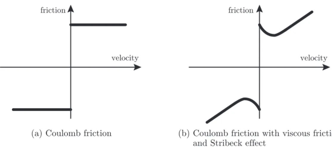
(a) Coulomb friction (b) Coulomb friction with viscous friction and Stribeck effect

Figure 1.1: Friction model represented by a function of which the output is determined uniquely with respect to the input velocity.

is affected by complicated factors such as inertia, Coriolis, centrifugal, gravity and friction forces, it is difficult to extract only the relation between the motion and the friction force.

Moreover in the case of assembled robots, the motion is limited by the joints’ mechanical limitation or the environment.

Even when we obtain an appropriate friction model, friction compensation is not still trivial problem, because we may not be able to estimate the friction state due to the limitation of the hardware such as the low resolution of the position sensors. There is possibility that the friction compensation based on the friction model is not sufficient, so a compensator that softens this problem is required.

One application of friction force estimation is external force estimation in which external force on a robot is estimated based on the equation of motion including a friction term. In this scheme, the accuracy of the external force estimation depends on the accuracy of the friction force estimation. Admittance control, which is one of force control schemes, is a further application of the friction (and external) force estimation.

1.2 Modeling of Friction

Many friction models have been proposed so far. One of simplest friction models is Coulomb

friction model [8, 31], which is usually represented by a function of which the output is de-

(a) Elastoplastic friction model (b) Parallel connection of friction element with spring and damper

Figure 1.2: Friction models containing presliding property.

termined uniquely with respect to the input velocity as Figure 1.1(a). This model has been combined with viscous friction, which increases with increasing velocity, and Stribeck ef- fect, which is friction property where the friction force decreases with increasing velocity.

These models capture the properties in the kinetic friction region well, but they cannot cap- ture properties in the static friction region, which is the neighborhood of zero-velocity where the models have the discontinuity.

Motivated by observation of small elastic displacement even in the static friction region, Dahl [16] has proposed a friction model that is schematically illustrated as Figure 1.2(a).

This model is a serial connection of a Coulomb friction element and an elastic component that corresponds to the elasticity of the contacting objects. The observed ‘presliding dis- placement’ is interpreted as the displacement by the elongation of the elastic element. At this time, the Coulomb friction element is stuck, so this region is called presliding region.

On the other hand, the region where the friction element is slipping is called sliding region.

Dahl has formulated this friction model by differential equations, and thus it can be regarded as ‘dynamic’ friction model.

After Dahl model, many dynamic friction models have been proposed. Canudas de Wit

et al. [10] have proposed LuGre model, which is a friction model that combines the Stribeck effect with Dahl model. This model captures friction phenomena such as stick-slip mo- tion, friction lag and varying break-away force. Swevers et al. [87] have presented Leuven model, which is an extension of LuGre model and has an arbitrary function for represent- ing hysteresis in the presliding region. Leuven model has been modified by Lampaert et al. [57] where the hysteresis function is implemented by a parallel connection of friction el- ements [26, 36, 45]. This formulation of friction is organized by Al-Bender et al. [1, 58], and is named the Generalized Maxwell Slip (GMS) model, which is illustrated as Figure 1.2(b).

The GMS model is one of the most famous friction models for its ability to capture many friction phenomena. Boegli et al. [6, 7] have improved the GMS model by smoothening the behavior of the model.

Other researchers also have been inspired by Dahl model. Hayward and Armstrong [32]

have proposed an elastoplastic friction model that is composed of a Coulomb friction ele- ment and an elastic element. The discretized algorithm of this model is derived by the ge- ometric relation of the input position and the friction element’s position. Dupont et al. [21]

have proposed a single state elastoplastic friction model with refined static friction behav- ior. Kikuuwe et al. [55] have considered the discrete time representation of an elastoplastic friction model, and they [56] have proposed discrete-time algorithms of visco-elastoplastic friction model, which is a generalization of Hayward and Armstrong’s elastoplastic friction model with non-zero viscosity. This discretization is an approximation of continuous-time representation of differential inclusion (i.e., differential equation including discontinuity) based on the backward Euler method. Xiong et al. [97] have derived a continuous differ- ential equation of visco-elastoplastic friction model from the original differential inclusion.

Xiong et al. [96] also have extended the single-state friction model to a multi-state one. Ad-

vantages of models of Kikuuwe et al. [55, 56] and Xiong et al. [96, 97] are the continuous

output friction force by excluding any discontinuous part.

1.3 Identification of Joint Friction

1.3.1 Sliding region and presliding region

In order to deal with joint friction in mechanical systems, it is necessary to identify the property and the magnitude of the friction. As mentioned above, friction phenomena have been formulated in the both of the sliding region and the presliding region by functions of which the output is determined uniquely with respect to the input or differential equations, and thus an identification method appropriate to each regime is necessary.

The relation between velocity and friction in sliding region is one of most remarkable properties from the viewpoint of control. Canudas de Wit and Lischinsky [9] have obtained velocity-friction curve of joints of a robot by observing the signal of the velocity and the actuator torque through tests commanding constant velocities, which has been used by other researchers [24, 34, 50]. Other schemes are based on sinusoidal [51] or saw-teeth [94] form force input. When methods mentioned above are applied to an assembled robot, there is possibility that the motion of the robot reaches the limitation by the configuration or envi- ronment, so we must consider the motion trajectory explicitly.

Identifying manipulator’s parameters such as inertia, gravity and friction simultane- ously is an interesting challenge for its potential to reduce the required time. Gautier et al. [67, 68, 83] have proposed identification methods based on an inverse dynamic model and least square regression. In such methods, the equation of motion of a manipulator is linearized with respect to the vector that contains the dynamical parameters, and the param- eters are identified by solving the linearized equation of which the components come from experimental data. In order to achieve efficient and successful identification, the parameters to be identified is reduced by eliminating parameters that have no effect on the dynamic model and by regrouping the parameters [25], and the trajectory of robot has been consid- ered to excite the properties such as inertia, gravity and friction [67, 68, 95]. Because these methods usually are targeted to many parameters, the formulation of friction term must be simple for low computational cost, which sacrifices the versatility of friction identification.

For further precise control, modeling and identification of joint friction in presliding

region is required. Canudas de Wit and Lischinsky [9] have identified nominal parameters

(stiffness and viscosity in presliding region) of LuGre model for a DC motor mechanism using a numerical optimization method based on the system model, and applied it to adaptive friction estimation and compensation. Rizos and Fassois [77, 78] have identified presliding friction of an actuator system based on Maxwell Slip model, i.e. a parallel connection of elastoplastic elements, by means of inverse dynamic model and least square regression. A similar method has been used for a harmonic drive transmission [89]. Iwatani et al. [42] have identified elastic coefficients of parallel visco-elastoplastic friction model for manipulator joints in which harmonic drives are embedded by physical interpretation between the model and experimental data. Because the frictional behavior is different between in the sliding region and in the presliding region, the identification also should be performed separately by appropriate ways for such regions.

1.3.2 On-line method

As with the identification methods mentioned above, friction identification should be ac- complished in advance in a basic sense. In the field of control, however, the identification is sometimes performed on-line, i.e., at the same time as a robot is doing its tasks, where the parameters are adjusted by adaptive methods. Canudas de Wit and Lischinsky [9] have proposed an adaptive friction estimation method based on nominal LuGre model with an additional parameter adjusting the output friction force. Tan and Kanellakopoulos [88] have extended Canudas de Wit and Lischinsky’s method [9] using multiple adaptive parameters.

Grami and Aissaoui [27] have proposed an on-line identification method for parameters of the GMS model. Ljung [63] have proposed a method to estimate parameters of a system on-line by recursive least square algorithm. Ruderman [79] have found a parameter set of friction of robotic joints based on the recursive least square method with the initial parameter set is determined in advance by a least square method.

Although adaptive methods have ability in adjustment, the accuracy of parameters iden-

tified in advance is still important, because the initial parameters may be set as the pre-

identified one.

1.4 Compensation of Joint Friction

Joint friction in robotic systems deteriorates the performance of the control. One straight- forward way to deal with such problem is friction compensation, i.e., making the effect of the friction smaller by generating the actuator force canceling the friction force.

A conventional proportional-integral-differential (PID) position controller has ability to suppress the effect of the friction with high stiffness by high gains. In unstructured environ- ment such as human workspace, however, high stiffness position control is not preferable because a system that includes such a controller does not have compliance and causes injury when it collides with human. Other control methods suppressing the effect of the friction have been proposed such as nonlinear PID position controllers [2, 80, 82] or sliding mode controllers [46, 85, 92, 93]. Such methods assume the desired position. It means that the controllers are connected with the controlled objects strongly and lack universal use.

The methodology of friction compensation on which this dissertation focuses is differ- ent from that of the controllers mentioned above. Friction compensation based on a friction model is advantageous because it does not need any desired value. Moreover, it has potential possibility to make joints free from friction. Such compensators are easy to superpose on any other controllers, and for situations where joint friction hampers the control, the com- pensators break through problems. This dissertation focuses on the advantage of the friction compensation based on a friction model.

1.4.1 Model-based compensation

In model-based friction compensation schemes, force estimated by a friction model is gen-

erated by the actuator to cancel the friction force. Coulomb friction model with viscous

friction and Stribeck effect has been used for compensation of friction in the sliding re-

gion [50,84]. For compensating friction in presliding region for robotic joints, LuGre model

has been utilized [9, 23, 35, 74]. Tjahjowidodo et al. [90, 91] have utilized the GMS model

for friction compensation control of a belt-driven DC motor system. Mahvash and Oka-

mura [66] have used Hayward and Armstrong’s [32] elastoplastic friction model for friction

compensation of tendon-driven joints. Iwatani et al. [42] have used a model composed of

parallel connection of Kikuuwe et al.’s [56] visco-elastoplastic friction model for friction compensation of harmonic drive gearings.

Some researchers have combined model-based friction compensation methods with other methods. Lee and Tomizuka [60] have proposed a friction compensation method based on Coulomb friction model and a disturbance observer for a position control system. Canudas de Wit et al. [9] have presented an adaptive friction compensation method based on Lu- Gre model for variation of friction of a position-controlled robotic system. In this method, the magnitude of the compensation force varies according to the position error. Lampaert et al. [59] have combined the GMS model and a disturbance observer using Kalman filter. Choi et al. [14] have developed a combination of a sliding mode controller and an extended LuGre model improved for pre-sliding hysteresis property. Maeda et al. [64, 65] enhances initial response of a disturbance observer by including bang-bang control or friction model-based compensation. Jamaludin et al. [43, 44] have combined a feed forward friction compensator based on the GMS model and a disturbance observer for control of a linear-drive feed table.

Zsch¨ack et al. [101] have proposed a friction compensation method based on GMS model adaptive for position-dependent friction.

1.4.2 Dither

For robotic joints with friction, some researchers [4, 29, 75] have focused on effectiveness of dither, i.e. high frequency oscillatory force by actuators. Dither is originally intended to improves the system smoothness by making the system in the kinetic friction state, where it is assumed that the friction force is smaller than in the static friction state. Stolt et al. [86]

have used dither for improving performance of external force estimation of a manipulator.

For robotic joints with high presliding stiffness, Aung et al. [5] have proposed a new dither

friction compensator, which is intended to make the system on the verge of the static friction

state and sensitive to applied force. Aung et al. [5] have combined the dither and model-

based friction compensation, and this method has successfully compensated the friction

in the presliding region, where only model-based method cannot compensate. Impulsive

control [3] is a similar method where small impulsive force is repetitively applied to the

system to produce positional modification in micro scale.

1.5 Estimation of Joint Friction Force

Estimating joint friction force, not compensating the friction, is also important. Friction force estimation requires only position sensors such as encoders, and in some scenes, only estimation of friction is sufficient. One of application of friction force estimation is external force estimation in which the external force acting on a robot is estimated based on the equation of motion that includes a friction term. External force estimators eliminate the need for force sensors, and the estimated force can be used for arbitrary controllers to maintain the safety of the system or to control the interaction force with the environment. Further application is admittance control, which is one of force control schemes.

One approach to estimate joint friction is a friction model, and another approach is usage of disturbance observers [30, 49, 62, 70, 73, 81], which is a method to estimate disturbance including friction. The fundamental concept is estimating unknown disturbance to a system by difference between the input and the output of the system. Chen et al. [11, 12] have proposed disturbance observers that contain nonlinear term. Nikoobin and Haghighi [71]

have proposed a nonlinear disturbance observer for a multi-link manipulator. Generally, disturbance observers contain noise reduction filters such as Butterworth low-pass filter, so their outputs usually include delay. Moreover, disturbance observers are based on the system model except disturbance, so the accuracy of the observers depends on the accuracy of the system model. Straightforward model-based friction estimation is advantageous, because a model-based method requires only a friction model and basically does not require any filter.

1.5.1 External force estimation

This section discusses external force estimation as an application of friction force estima-

tion. There have been many approaches of external force estimation of robots. A conven-

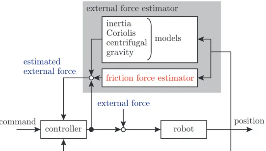
tional structure of external force estimation is illustrated in Figure 1.3, where the estimated

value is obtained based on inverse dynamics model including inertia, Coriolis, centrifugal,

gravity and friction term. Some researchers [48,72] have proposed external force estimation

methods based on disturbance observers, which regard the external force as the output of

disturbance observers subtracted with friction force. Li et al. [61] have applied an external

controller command

external force

robot position

estimated external force

inertia Coriolis centrifugal gravity

models

friction force estimator external force estimator

Figure 1.3: Robotic system including friction force estimator.

force estimator based on a disturbance observer to a teleoperated invasive surgical forceps manipulator to send the contact force back to the user. De Luca et al. [18, 19, 28] have de- veloped a method to detect collision between an industrial manipulator and the environment based on the momentum of the manipulator, where the collision is detected as estimated external force, and they have utilized the detection method to make manipulators produce safe reaction to soft objects and human bodies. An external force estimation method using joint torque sensors has been proposed by Phong et al. [76]. Colome et al. [15] have de- veloped an external force estimator of a compliant joint robotic manipulator, which employ a function mapping the relation between the state (position and velocity) and the external force obtained by a learning technique. Daly and Wang [17] have used an external force estimator for control of a bilateral teleoperation manipulator system.

Researchers have dealt friction terms in external force estimators by using simple fric-

tion models or employing other estimation methods despite of existence of many analytical

friction models. There is a potential possibility to improve the performance of external force

estimators by explicitly considering the friction terms.

external force estimator

admittance controller command

external force robot

position estimated external force

(b) With an external force estimator force sensor

admittance controller command

external force

robot

position measured force

(a) With a force sensor

Figure 1.4: Robotic system including admittance controller.

1.5.2 Sensorless admittance control

Admittance control [33] is one of force control schemes that intend to produce robot motion

achieving a desired admittance, where the word admittance means the relation between the

input force and the output velocity. This is also one of applications of friction (external)

force estimation techniques. In admittance control systems, the external force is usually

measured by force sensors as shown in Figure 1.4(a). Such methods are utilized for ex-

oskeleton robots [99], humanoid robots [100] and electric power steerings [98]. The use of

friction (external) force estimators allows us to eliminate the need for force sensors, which

have fragileness, high cost, and small sensible parts. The structure of sensorless admittance

control system is shown in Figure 1.4(b). External force estimation based on disturbance ob-

servers has been used in force control of a multi degree of freedom manipulator [69] and an

injection molding machine [72]. Erden and Tomiyama [22] have proposed a sensorless ad- mittance controller with an external force estimator for a robotic manipulator. In sensorless admittance control, the behavior of the controlled system strongly depends on the accuracy of the force estimation, which also depends on the treatment of the internal friction term.

1.6 Major Achievements

This dissertation is a contribution to handling friction of robotic manipulators by developing an identification procedure, a compensator and an estimator of friction. The major achieve- ments are as follows:

• Identification procedure for rate-dependent friction law (Chapter 2)

This dissertation proposes a procedure for identifying rate-dependent friction of robotic manipulators of which the motion is limited due to the configuration or the environment.

The procedure is characterized by the following three features: (i) the rate dependency is represented by line sections connecting sampled velocity-force pairs, (ii) the robot is position-controlled to track desired trajectories that are some cycles of sinusoidal motion with different frequencies, and (iii) each velocity-force pair is sampled from one cycle of the motion with subtracting the effects of the gravity and the inertia. The procedure was tested with a six-axis industrial robotic manipulator Yaskawa MOTOMAN-HP3J, of which the joints are equipped with harmonic-drive transmissions. The experimental re- sults show that the identification is achieved with a sufficient accuracy with the 20 degrees of motion of each joint. In addition, the results were utilized for friction compensation, successfully reducing the effect of the friction by 60 to 80 percent.

• New elastoplastic friction compensator (Chapter 3)

Mahvash and Okamura’s elastoplastic friction compensator is one of successful friction

compensators for robotic joints with compliant transmissions. A limitation of the scheme

is that, in the static friction state, the compensator continues commanding non-zero out-

put force, which hampers the system’s reaction to external forces. This dissertation

presents an improved version of the elastoplastic friction compensator with an additional

term, which makes the output force decay exponentially in the static friction state. The proposed method was tested using a linear actuator system with a ball screw and a timing belt and an industrial manipulator Yaskawa MOTOMAN-HP3J. The experimental re- sults show that the proposed method reduces external force required to move the device.

Further improvement of the compensator is also presented for ‘hand-drivabilization.’

• New elastoplastic friction estimator (Chapter 4)

This dissertation proposes an elastoplastic friction estimator with improved static fric- tion behavior for the applications of external force estimation and sensorless admittance control. Hayward and Armstrong’s elastoplastic friction model is one of the simplest model representing friction phenomena with compliance. This model however produces non-zero output force in the static friction state, which results in steady-state error in external force estimation. This chapter proposes a friction force estimator with the out- put force being reduced in the static friction state. The proposed estimator was tested through experiments with an actuator system comprised of a ball screw and a timing belt, and an industrial manipulator MOTOMAN-HP3J, Yaskawa Electric Corporation.

The experimental results show that the estimation accuracy is improved by the proposed estimator. The friction fore estimator is further improved for admittance controller with the estimator.

1.7 Organization

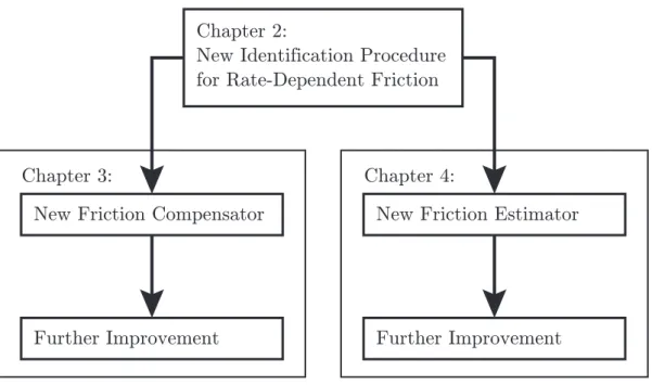
The connection between each chapters in this dissertation is illustrated as shown in Fig-

ure 1.5. The rest of this dissertation is organized as follows. Chapter 2 proposes a new

identification procedure for rate-dependent friction in manipulator joints. Chapter 3 pro-

poses a new friction compensator. Chapter 4 proposes a new friction force estimator. Note

that joint friction in setups used in Chapter 3 and 4 was identified by the procedure of Chap-

ter 2. Finally, Chapter 5 provides a concluding remarks.

Chapter 2:

New Identification Procedure for Rate-Dependent Friction

New Friction Compensator

Chapter 3: Chapter 4:

New Friction Estimator

Further Improvement Further Improvement

Figure 1.5: Interconnection among chapters.

Identification of Joint Friction:

Identification Procedure for Robotic Joints with Limited Motion Ranges

2.1 Introduction

For the control of robotic manipulators, friction in the joints is one of major disturbances that degrade the accuracy and the precision of control. One straightforward idea to deal with this problem is to calibrate the friction properties of the robot in advance and to compensate the friction force by producing the actuator forces that cancel the friction forces. It is how- ever usually difficult to find appropriate models of the friction phenomena and, even if an appropriate model is available, it is also difficult to clarify how the values of the parameters should be chosen.

Many friction models have been proposed so far, and they vary in the treatment of the discontinuity around the zero velocity and the microscopic elastic displacement in the static friction. A common point shared by various friction models is that they employ a user- defined function of velocity that represents the rate-dependent friction law. That is, for any

The content of this chapter is partially published in [40], namely, M. Iwatani and R. Kikuuwe. An Identification Procedure for Rate-Dependency of Friction in Robotic Joints With Limited Motion Ranges.

Mechatronics, 36:36–44, 2016.

15

kinds of friction models, the magnitude of the friction force as a function of the velocity must be identified experimentally.

Experimental identification of the rate dependency of the friction force is not always an easy task. Problems such as the limited motion range and the effects of the gravity and the inertia make the identification complicated. The motion of an assembled robotic manipu- lator is generally limited by the configuration or the environment. Appropriate procedures are needed to measure the friction force at high velocities in a limited motion range, and the identification results need to be insensitive to the effects of inertia and gravity.

This chapter presents a systematic procedure to identify the velocity-friction force rela- tion of devices with limited motion range. The procedure was validated with an industrial six-joint manipulator Yaskawa MOTOMAN-HP3J. It is shown that the identification with a sufficient accuracy was achieved with 20 degrees of motion of the joints. This chapter also shows the application of identified results to friction compensation.

The remainder of this chapter is organized as follows. Section 2.2 overviews previous studies on identification of rate-dependent friction. Section 2.3 proposes the new proce- dure. Section 2.4 and 2.5 show experimental results obtained with a six-axis manipulator.

Section 2.6 provides concluding remarks.

2.2 Related Work

Many friction models have been proposed for the purpose of control. They have realized

friction property such as rate-dependency in the kinetic friction [4], elastic displacement

in the static friction [16], hysteresis in the velocity-friction relation, stick slip motion [10],

non-drifting [1, 87], and smoothness of the output force [96]. Discrete-time models have

also been considered [32, 56]. There have been applications of the models to friction com-

pensation [50, 87], and harmonic drive transmissions especially have been the target of ap-

plications of modeling studies [5, 20, 42, 91]. One common feature shared by many models

including dynamic friction models is that they employ functions of velocity for representing

the rate-dependent friction force in the kinetic friction region. It means that the velocity-

friction relation must be calibrated in advance for using any kinds of existing models in-

cluding dynamic friction models.

Rate-dependent friction of manipulators can be identified by maintaining a constant ve- locity for a certain period of time [24, 50]. In such methods, constant velocity commands are sent to the devices, and the resultant actuator torque to maintain the velocity is observed.

One drawback of such methods is that maintaining high velocity is generally difficult within a limited range of motion. Another kind of approach is to apply sinusoidal or saw-tooth torque signals to devices to be identified [51, 94]. Such torque command, resulting recip- rocating motion, requires a certain level of carefulness in choosing the torque amplitudes so that the trajectory of motion is bounded to a limited range. As mentioned above, the limitation of motion in joints is problematic for identification of rate-dependent friction, so we need a method explicitly handling the limitation of motion.

The gravity and the inertia affect the accuracy of the identified results. A straightforward idea to deal with these factors is to incorporate a system model including the gravity and the inertia into the identification procedure [13,50,51,94]. Major drawbacks of this approach are that the identification of the system model is usually a hard task, and that the identification accuracy of the friction depends on the accuracy of the whole system model.

2.3 Procedure

2.3.1 Overview

This section describes a new identification procedure for rate-dependent friction laws. The procedure is to obtain a set of N velocity-force pairs

S =

{ [V

, F

], · · · , [V

, F

] } , (2.1)

which describes the relation between the velocity and the friction force as shown in Fig-

ure 2.1. The joint to be identified is controlled to follow sinusoidal trajectories with N

different frequencies with a high-gain PID position controller. One cycle of motion is per-

formed for each frequency. The pair [V

, F

] is chosen so that the effects of inertia and

gravity are small. The identification on each joint is performed on a one-by-one basis, with

F

{ V

v

Á ( v )

F

F

F

V

V

V

{ F

{ F

{ F

{ F

{ V

{ V

Figure 2.1: Fitted curve φ(v) defined by (2.8).

the other joints being locked by local position controllers.

2.3.2 Details

The input to the procedure is the following three parameters:

• V : The maximum desired velocity

• A : The amplitude of the sinusoidal motion

• N : The number of sampled velocities

The maximum velocity V should be chosen so that it includes the range of velocity in

which the friction force should be identified. The amplitude A should be chosen small

enough to match the hardware limitation, and should be smaller to save the time needed for

the identification procedure. Its lower bound is determined by the capacity of the actuator

because, with a fixed V value, the desired acceleration command is inversely proportional to

the A value, as will be shown later. The number N of sampled velocities should be chosen

considering the trade-off between the precision of the fitted curve and the time needed for

the identification.

desired position p

time t

T

A

V V N

time t

T

T

T

T

desired velocity v

2 V

N

¼AN V ¼AN 2 V

Figure 2.2: Desired trajectory p

(t) and its derivative v

(t) for the proposed identification procedure.

As one of the simplest position trajectories to obtain the set S of velocity-force pairs, the following desired position trajectory has been chosen:

p

(t) =

A 2

1 − cos

2ν(t)V

AN (t − T

)

(2.2) where

T

=

j=1

πAN

jV (2.3a)

ν(t) =

n s.t. t ∈ T

= [T

, T

). (2.3b) This position trajectory p

(t) is based on the following velocity trajectory:

v

(t) =

ν(t)V N sin

2ν(t)V

AN (t − T

)

. (2.4)

These trajectories p

(t) and v

(t) are illustrated in Figure 2.2. Here, it can be seen that p

(t) is composed of N times of sinusoidal movements with N different frequencies. The amplitude of the desired position p

is fixed to A, and the maximum velocity of the nth cycle is nV /N. It should be noted that the amplitude of v ˙

is proportional to V

/A, and thus the choice of the A value is lower-bounded by the capacity of the actuator. If the chosen A value is too small, the manipulator will not be able to track the resultant desired trajectory, but it will not cause any damage on the hardware and will need only a retry of the procedure with a larger A value. This feature is in contrast to torque-based [51, 94] or velocity-based [24, 50]

identification schemes, in which inappropriate parameter design may result in the hardware damage.

Once the joint is position-controlled to track the aforementioned desired trajectory, the data as shown in Figure 2.3 is expected to be obtained. Here, it is advisable that the gains of the position controller should be set as high as possible. The control accuracy however only needs to be enough to realize the velocity above the maximum desired velocity V , which is given as a parameter of the procedure. This is because what is important here is the relation between the applied force f and the actual velocity v, which describes the physical property of the joint, and is not the relation between v and the desired velocity v

. With a sampling interval Δt, the measured velocity v

and the applied force f

are obtained at the time t

where i ∈ { 1, · · · , I } and

I =

T

/(Δt). (2.5)

Consequently, an experiment in the presented procedure provides the following sets of data:

T

= { t

, t

, · · · , t

}

V

= { v

, v

, · · · , v

} (2.6) F

= { f

, f

, · · · , f

} .

The data {T

, V

, F

} can be utilized to obtain the set S through the following function:

FunctionA( T

, V

, F

) (2.7a)

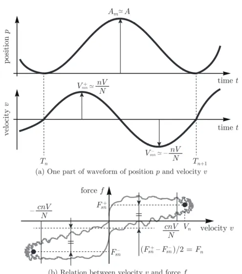
position pvelocity v

(a) One part of waveform of position p and velocity v

velocity v force f

(b) Relation between velocity v and force f F ^{ (F ⁺ {F ^{ )/2 = Fn

N { cnV

sn sn sn

time t

time t

T_n T_n+1

A Am

Fsn ⁺

N cnV Vn

V ^{mn { N nV V ^+mn

N nV

Figure 2.3: Schematic illustration of data that could be obtained from the procedure.

for n := 1 to N (2.7b)

V

:= { v

∈ V

| t

∈ T

∧ v

≥ cnV /N } (2.7c) F

:= { f

∈ F

| t

∈ T

∧ v

≥ cnV /N } (2.7d) F

:= { f

∈ F

| t

∈ T

∧ v

≤ − cnV /N } (2.7e)

V

:= Average( V

) (2.7f)

F

:= Average( F

) (2.7g)

F

:= Average( F

) (2.7h)

F

:= (F

− F

)/2 (2.7i)

end for (2.7j)

S := { [V

, F

], · · · , [V

, F

] } (2.7k)

Return S . (2.7l)

Figure 2.3(b) illustrates the relations among some variables that appear in this procedure.

Here, Average( X ) is a function that returns the average value of the elements of input set X . The ratio c ∈ [0, 1) determines the boundaries of the range of the sampled data used for the identification, by multiplying the maximum desired velocity nV /N in each cycle as can be seen in (2.7c)-(2.7e) and Figure 2.3. The ratio is set at c = 0.8 in this chapter.

Now, the set S is obtained through algorithm (2.7). Based on the set S, the rate- dependent friction is defined as the following function φ(v):

f = φ(v) = sgn(v)

B

( | v | − V

) + F

(2.8) where

B

= (F

− F

)/(V

− V

) (n ∈ { 1, · · · , N − 1 } ) (2.9a)

B

=

B

(2.9b)

B

=

B

(2.9c)

V

= 0

(2.9d)

V

= +

∞ (2.9e)

F

=

F

− B

V

(2.9f)

n(v ) =

n s.t. V

≤ v < V

. (2.9g)

The function is illustrated in Figure 2.1. It is a combination of line sections connecting the

elements of the set S, and is symmetric with respect to v = 0 . Note that all parameters

{ B

, V

, F

} are derived from the set S .

p M L

locked focused

Figure 2.4: Schematic illustration of robot regarded as a 1-link manipulator.

2.3.3 Analysis on the influence of inertia and gravity

The algorithm in this chapter uses only the data near the velocity peaks, and estimates the friction force by taking the semi-amplitude of the force values at the velocity peaks. This is based on the intention to minimize the effects of the inertia and the gravity to the estimated friction force F

as explained by the following.

Let us regard the robot as a 1-link rotational manipulator because the joints except the focused one are locked as shown in Figure 4. Then, the actuator force f can be represented as follows:

f = f

( ˙ p) + I p ¨ + M Lg cos(p) (2.10) where f

(v) is the rate-dependent friction force, I is the moment of inertia around the joint, M is the total mass, L is the length from the joint to the center of mass (COM), p is the angle between the horizontal surface and the line passing through the joint and the COM, and g is the gravity acceleration.

As has been explained in Section 2.3.2, the angle p can be given as a sinusoidal function of time t as follows:

p = p

+ A cos(ωt) (2.11)

where A and ω are the amplitude and the angular frequency of the motion and p

is a con-

stant, respectively. Then, (2.10) can be rewritten as follows:

f = f

(Aω sin(ωt)) − IAω

cos(ωt) + M Lg cos (p

+ A cos(ωt)) (2.12) The force values F

and F

at the velocity peaks can be written by (2.12) with t = π/(2ω) and 3π/(2ω) as follows:

F

= f

(Aω) + M Lg cos (p

) (2.13a) F

= f

( − Aω) + M Lg cos (p

) (2.13b) Substituting (2.13a) and (2.13b) for (2.7i) yields the following equation:

F

= (f

(Aω) − f

( − Aω)) /2 f

(Aω) (2.14) because of the assumption that the rate-dependent friction force is symmetric with respect to v = 0, that is, f

( − Aω) − f

(Aω).

What (2.14) implies is that F

does not depend on the inertia term I p ¨ or the gravity term M Lg cos(p

) . This can be explained by the fact that the acceleration is close to zero at the velocity peaks and the angle joint at the two velocity peaks are close to each other.

2.4 Experiment: Identification

2.4.1 Experimental setup

The proposed identification procedure was experimentally tested with a six-axis robotic ma- nipulator Yaskawa MOTOMAN-HP3J shown in Figure 2.5. A harmonic drive transmission is embedded to each joint. Table 2.1 shows the specification of each joint. A force sensor NITTA IFS-50M31A25-I25 is attached at the end-effector to measure the external force in experiments of friction compensation to which the identified results are applied.

The experimental comparison with methods in literature is not included in this chap-

ter. The proposed method is based on the position control, which is intrinsically capable

(a) MOTOMAN-HP3J

0

5 4 3 2

1

(b) Configuration force sensor

Figure 2.5: Experimental setup.

Table 2.1: Specification of the experimental setup.

Joint number [-] 0 1 2 3 4 5

Reduction ratio [-] 100 224 120 120 100 81.5

Maximum velocity [deg/s] 200 135 190 250 300 360 Maximum torque [Nm] 95.1 213.1 114.1 34.2 28.5 23.3

of limiting the joint motion within the mechanical limitations. In contrast, other methods

are based on torque command [51, 94] or velocity command [13, 24, 50], and thus there is

the possibility that the motion of the joint arrives in the mechanical limitation. Therefore,

experiments under the same condition cannot be performed. Previous methods focused

on, for example, identification in low velocity range [50], position-dependent friction [24],

dynamic friction models [51], nonlinear optimization problem [94], or identification using

transfer functions [13].

-¹⁰⁰ -^{50 0 50 100} -¹⁵⁰

-¹⁰⁰ -⁵⁰ 0 50 100

150 A = 10 deg

-¹⁰⁰ -^{50 0 50 100} -¹⁵⁰

-¹⁰⁰ -⁵⁰ 0 50 100

150 A = 30 deg

-¹⁰⁰ -^{50 0 50 100} -¹⁵⁰

-¹⁰⁰ -⁵⁰ 0 50 100 -¹⁰⁰ -^{50 0 50 100} 150

-¹⁵⁰ -¹⁰⁰ -⁵⁰ 0 50 100

150 A = 20 deg

torque f [Nm]

-¹⁰⁰ -^{50 0 50 100} -¹⁵⁰

-¹⁰⁰ -⁵⁰ 0 50 100 150

Others experimental results identified curve f = Á(v)

A = 50 deg A = 40 deg

angular velocity v [deg/s]

torque f [Nm] torque f [Nm]torque f [Nm]torque f [Nm]

angular velocity v [deg/s]

Figure 2.6: Experimental results and the identified curves in the cases of various A at Joint 1.

Experimental results are unbiased.

2.4.2 Sensitivity to the choice of A

It is desirable to set A as small as possible for reducing the time needed for the identification, because the time required for tracking the trajectory (2.2) is proportional to A as shown in the following equation:

T

= πAN V

1

j , (2.15)

-

-

-

-

-

-¹⁰⁰ -^{50 0 50 100} -⁵

0 5

-¹⁰⁰ -^{50 0 50 100} -⁴

-² 0 2 4

-

-

-

-

-

-

-

-

-¹⁰⁰ -^{50 0 50 100} -⁴

-² 0 2 4

Joint 0

Joint 2

Joint 1

Joint 3

Joint 5

A = 5 deg

A = 10 deg

A = 10 deg

A = 5 deg

A = 5 deg A = 5 deg

A = 5 deg A = 10 deg

A = 10 deg A = 10 deg

A = 5 deg A = 5 deg

A = 10 deg

Joint 4

A = 5 deg

A = 5 deg

torque f [Nm]torque f [Nm]torque f [Nm]

torque f [Nm]torque f [Nm]torque f [Nm]

angular velocity v [deg/s] angular velocity v [deg/s]

A = 50 deg A = 40 deg A = 30 deg A = 20 deg A = 10 deg A = 5 deg

Figure 2.7: Identification results of each joint in various cases of A under V = 115 deg/s

(2.0 rad/s) and N = 10 . The result in the case of A = 5 deg at Joint 1 was not obtained due

to the limit of the servo controller.

Joint 0

5 10 20 30 40

E(A,50) [Nm]

0.0 0.5 1.0 1.5 2.0

Joint 2

5 10 20 30 40

0.0 0.2 0.4 0.6 0.8 1.0 1.2

E(A,50) [Nm]

Joint 4

5 10 20 30 40

0.00 0.05 0.10 0.15

E(A,50) [Nm]

Joint 1

5 10 20 30 40

0.0 0.5 1.0 1.5 2.0

E(A,50) [Nm]

Joint 3

5 10 20 30 40

0.0 0.2 0.4 0.6 0.8 1.0 1.2

E(A,50) [Nm]

Joint 5

5 10 20 30 40

0.00 0.05 0.10 0.15

E(A,50) [Nm]

value of A [deg] value of A [deg]

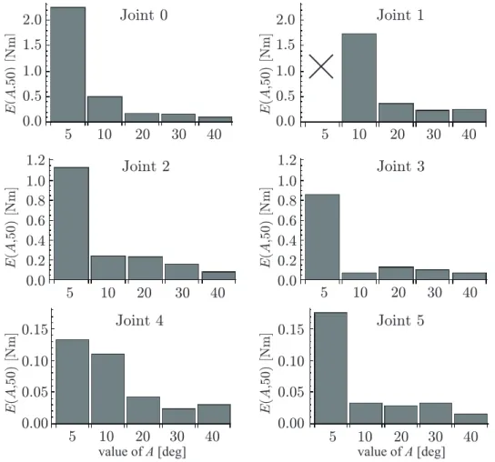
Figure 2.8: Difference between each curve and the curve of A = 50 deg based on (2.16) under V = 115 deg/s (2.0 rad/s) and N = 10. The symbol × means that the result was not obtained due to the limit of the servo controller.

which can be seen in (2.3) and Figure 2.2. Figure 2.6 shows experimental results and iden- tified curves with various values of A, under V = 115 deg/s (2.0 rad/s) and N = 10.

Figure 2.6 is the result of Joint 1, where the effect of the gravity and the inertia is the largest among all joints. The bias of each experimental result is removed to make it comparable to the fitted curve φ(v) obtained by the proposed procedure. It can be seen that smaller A , resulting larger effect of inertia, broadens the width of the curves and also perturbs the fitted curve φ(v). Therefore, it can be concluded that too small A deteriorates the accuracy of the identification. The following shows how small A can be at each joint.

Figure 2.7 is the identified results with various A at each joint. In this figure, one can see

that the curves of A larger than 10 deg are almost overlapping. Thus, it can be said that the amplitude of trajectory A = 20 deg is enough to identify the friction curve appropriately.

Moreover, it is clear that the slope of the identified curves in the high velocity range is different from that in low velocity range. This indicates that the high velocity range should also be identified experimentally, not only by extrapolation.

In order to validate the results quantitatively, we use the following distance metric:

E(A

, A

) =

1 V

0

(φ

(v ) − φ

(v))

dv. (2.16) This metric represents the difference between the curves φ

(v) and φ

(v ) that are obtained with A = A

and A

respectively. Figure 2.8 shows the quantitative difference between each curve and the curve of A = 50 deg at each joint. It is shown that the differences are large when A = 5 or 10 deg. These results correspond to Figure 2.7, quantitatively indicating that the trajectory amplitude of A = 10 or 20 deg is the minimum necessary value for appropriate identification, under the condition of the range of velocity V = 115 deg/s (2.0 rad/s) in the device MOTOMAN-HP3J.

One limitation of the scheme is that the identified curve is always a continuous function of velocity except the zero velocity. This issue however should not be viewed as a critical problem for many lubricated actuators because, in such mechanisms, the static friction state and the kinetic friction states are continuously connected through the Stribeck effect.

2.4.3 Sensitivity to the posture

Another set of experiments were carried out to show the effects of inertia and gravity on the

identification results. The identification was performed on Joint 1 with five different postures

shown in Figure 2.9(a) under the condition of A = 20 deg, V = 115 deg/s (2.0 rad/s) and

N = 10. The different postures yield the different inertia and gravity force with respect to

the joint. Figure 2.9(b) is the identification results, which show that the curves are almost