Stability and bifurcations of two-dimensional zonal jet flows on a rotating sphere
By
Eiichi SASAKI
January 2013
R ESEARCH I NSTITUTE FOR M ATHEMATICAL S CIENCES
Stability and bifurcations of two-dimensional zonal jet flows on a rotating sphere
Eiichi SASAKI
Research Institute for Mathematical Sciences, Kyoto University
In planetary atmospheres in Jupiter or Saturn, for example, strong zonal jets have been observed. The existence of the zonal jet flow has been considered as one of the robust properties of planetary atmospheres.
The two-dimensional incompressible Navier-Stokes flow on a rotating sphere is con- sidered to be one of the simplest and most fundamental models of the atmospheric motions taking into account the effect of the planetary rotation. The Reynolds number of the plan- etary atmospheres is so large that properties of the Navier-Stokes turbulence on a rotating sphere should be relevant to some aspect of the dynamics of the atmosphere. However, even in this simplest model, it is far from straightforward to obtain global properties of fully nonlinear solutions. In this thesis we discuss the Navier-Stokes flows on a rotating sphere, with an attention focused on the stability problem, the bifurcation structure of the zonal jet flows and chaotic solutions at high Reynolds numbers.
First we show the inviscid stability of the zonal jet flows on a rotating sphere. The semi-circle theorem obtained by Howard (1961) on a non-rotating planer domain is extended to the rotating sphere. We also study the linear stability of the zonal jet flows (l-jet flow) the streamfunction of which is expressed by a single spherical harmonics function Yl0. This linear stability problem was first studied by Baines (1976), and his numerical result has been considered as a standard result for the zonal jet flows. We show that the critical rotation rates obtained by Baines include numerical errors caused by an emergence of singularities (critical layers), and we give accurate numerical results for the critical rotation rate by using a power-series expansion and a shooting methods taking into account the singular points.
Next, we study the viscous stability problem and the bifurcation diagram of the zonal jet flows, by introducing a forcing term balancing with the viscous dissipation terms.
This setting is similar to the Kolmogorov problem, in which the stability and the bifurcation diagram of two-dimensional Navier-Stokes flows on a flat torus is considered. We prove rigorously that the 2-jet zonal flow is globally and asymptotically stable for an arbitrary Reynolds number and rotation rate. Then we study the linear stability of l-jet zonal flow for l ≥3 and find an interesting phenomenon that the inviscid limit of the critical stability point does not coincide with the inviscid critical stability point. We also show that this is not a contradiction because the inviscid limit of the growth rates of the viscous unstable modes coincides with that of the inviscid unstable mode. In the numerical simulation by Obuse et al. (2010), the asymptotic states of forced two-dimensional turbulence are only the 2- or 3-jet zonal flows. A discussion is given on their results and our result on stability of laminar jets.
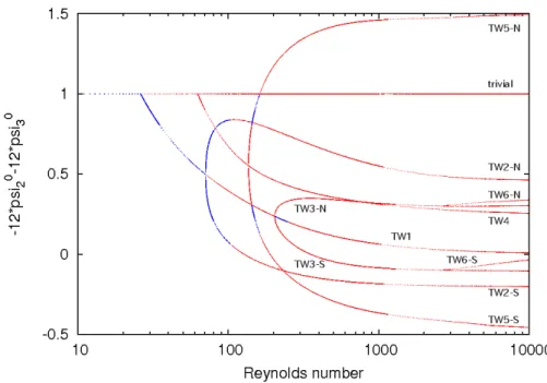
We study the bifurcation structure arising from the 3-jet zonal flow. In non-rotating case, at the critical Reynolds number, a steady traveling wave solution arises from the 3-jet zonal flow through the Hopf bifurcation. As the Reynolds number increases, several traveling solutions arise only through the pitchfork bifurcations and at high Reynolds numbers the steady bifurcating solutions become Hopf unstable. For the steady bifurcating solutions in
the non-rotation case, we find symmetry restoration of the streamfunction at high Reynolds numbers. Similar phenomenon has been found in Kolmogorov problem by Okamoto and Sh¯oji (1993) and Kim and Okamoto (2010). In the rotating case, on the other hand, we find the saddle-node bifurcations and a closed-loop branch. These results show that the bifurcation structure changes drastically, as the absolute value of the rotation rate increases.
We also carry out time integration of unsteady zonal flows at high Reynolds num- bers on the non-rotating/rotating sphere. We reproduce the zonal-mean zonal velocity of the unsteady solution from those of the unstable steady and steady traveling solutions by making a linear mapping from the solution space to the zonal-mean zonal profiles. In the non-rotating case, we find that the solutions are chaotic, and the reproduction of the zonal-mean profiles is satisfactory although the linear mapping assumes the linear inter- and extra-polation of the profile of the steady and steady traveling solutions in the solution space. However, in the rotating cases, the solution tends to be less chaotic under the stabilizing effect of rota- tion, and we find that the reproduced zonal flow by the linear mapping method does not approximate well the zonal-mean zonal velocity of the solutions. These results suggest that in the non-rotating case even the chaotic orbits at high Reynolds number lies mostly within a relatively low-dimensional box, the vertices of which are the steady and steady traveling solutions, and in the rotating case the relation between the unsteady solutions and the steady or steady traveling solutions changes as the effect of rotation increases.
1 Introduction 9
1.1 Planetary atmospheres and two-dimensional fluids . . . 9
1.2 Two-dimensional turbulence in a plane . . . 10
1.3 Effect of rotation on two-dimensional turbulence . . . 10
1.4 Two-dimensional turbulence on a rotating sphere . . . 11
1.5 Inviscid stability problem of zonal jets . . . 11
1.6 Viscous stability of the zonal jets and Kolmogorov problem . . . 12
1.7 Results of the present study . . . 14
2 Stability of inviscid zonal jet flows on a rotating sphere 16 2.1 Introduction . . . 16
2.2 Governing equations . . . 17
2.3 Semi-circle theorem . . . 18
2.4 Re-examination of the stability of inviscid zonal flow . . . 20
2.4.1 Stability analysis with a spectral method . . . 20
2.4.2 Stability analysis with a shooting method . . . 22
2.5 Conclusion and Discussion . . . 28
3 Stability and bifurcation structure of viscous zonal jet flows on a rotating sphere 30 3.1 Introduction . . . 30
3.2 Governing equations . . . 31
3.3 Global stability of 2-jet zonal flow . . . 33
3.4 Linear stability of thel-jet zonal flows . . . 35
3.5 Bifurcation structure of nonlinear steady solutions arising from 3-jet zonal flow 41 3.5.1 Bifurcation diagram in the non-rotating case . . . 42
3.5.2 Bifurcation diagrams in the rotating case . . . 42
3.5.3 Characteristics of steady traveling solutions at high Reynolds number 48 3.6 Numerical simulations at high Reynolds number under 3-jet zonal forcing . . 51
3.6.1 Properties of chaotic solutions in the non-rotating case . . . 51
3.6.2 Properties of solutions orbits in the rotating case . . . 61
CONTENTS 3.7 Conclusion and Discussion . . . 67
4 Conclusion 70
2.1 Eigenvalues of linear stability of inviscid 3-jet zonal flow. . . 21
2.2 Unstable eigenvalues around Ω = Ω−B. . . 22
2.3 Vorticity of the unstable eigenfunctions at Ω = Ω−B. . . 23
2.4 Unstable eigenvalues around Ω = Ω+B. . . 23
2.5 Vorticity of the unstable eigenfunction at Ω = Ω+B. . . 24
2.6 Schematic of the integral path on the complex plane. . . 26
2.7 Stability eigenvalues around the negative critical rotation rate. . . 28
3.1 Critical Reynolds number of l-jet zonal flow in the non-rotating case. . . . . 36
3.2 Neutral curves and real part of phase velocity of 3- and 4-jet zonal flow on R-Ω plane. . . . 38
3.3 Growth rates of the most unstable mode of 3-jet zonal flow. . . 40
3.4 Growth rates of the most unstable mode in regions of inviscid zonal flow is stable while viscous zonal flow is unstable. . . 40
3.5 Streamfunction and longitudinal velocity of 3-jet zonal flow. . . 41
3.6 Bifurcation diagram at Ω = 0.0 . . . 43
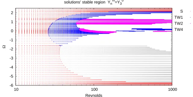
3.7 Stable regions of nonlinear steady solutions on R-Ω plane. . . . 44
3.8 Bifurcation diagram at Ω =−0.5 and −1.0. . . 46
3.9 Bifurcation diagram at Ω = 0.5 and 1.0. . . 47
3.10 Streamfunctions of TW1 at high Reynolds number. . . 49
3.11 Zonal-mean zonal velocity of TW1 and TW5 at Ω = 0.0. . . 50
3.12 Streamfunctions of TW5 at Ω = 0.0. . . 50
3.13 Streamfunctions of nonlinear steady solutions at Ω = 0.0 and R= 104. . . . 52
3.14 Zonal-mean zonal velocities of nonlinear steady solutions at Ω = 0.0 and R= 104. . . 52
3.15 Time series and power spectrum of energy density of the chaotic orbits. . . . 53
3.16 Snapshots of streamfunction of chaotic solution at Ω = 0.0 and R= 104. . . 54
3.17 Snapshots of zonal-mean zonal velocity of chaotic solution at Ω = 0.0 and R= 104. . . 54
3.18 Zonal-mean zonal velocity of the chaotic orbits. . . 55 3.19 Reproduction of time-averaged zonal-mean zonal velocity of the chaotic orbits. 57
LIST OF FIGURES 3.20 Zonal-mean zonal velocity obtained by the linear mapping using a single
steady/steady traveling solution. . . 59
3.21 The time series of the error of the approximation. . . 59
3.22 Ensemble-time-averaged error of the approximation. . . 60
3.23 Time-mean and ensemble-mean relative error of the linear mapping. . . 63
3.24 Power spectrum of the energy density of unsteady solutions at Ω = 0.0,±0.5,±1.0 with R= 103,104. . . 64
3.25 Streamfunctions of nonlinear steady solutions at Ω =−1.0 and R= 103. . . 65
3.26 Snapshot of chaotic solution at Ω =−1.0, R = 103. . . 65
3.27 Snapshot of quasi-periodic solution at Ω =−1.0, R = 103. . . 65
3.28 Reproduction of time-averaged zonal-mean zonal velocity of the time-periodic solution at Ω =−1.0, R = 103. . . 66
2.1 Critical rotation rates of inviscid l-jet zonal flows. . . . 27
3.1 Lowest critical Reynolds number of l-jet zonal flow. . . . 37
3.2 Critical rotation rates of viscous l-jet zonal flows. . . . 39
3.3 The solutions used in the linear mapping . . . 62
3.4 The type of solutions obtained by time integration. . . 66
Chapter 1 Introduction
1.1 Planetary atmospheres and two-dimensional fluids
Dynamics of fluid motion of human size have been investigated for over one hundred years, and fruitful insights in fluid motions have been obtained together with new attractive prob- lems by experimental and theoretical studies. We now have rich knowledge about a set of simple fundamental flows which serve as components of complex fluid motions encountered in daily life. Recently, large-scale fluid phenomena in planetary atmospheres has been ob- servable by using satellites and high-performance telescopes. However, the observational data is still quite lacking, and experimental study of most of these flows is impossible. The understanding the large-scale flows are therefore far from satisfactory compared to the flows in daily life, and our knowledge is quite limited even about simplest fundamental flows.
In planetary atmospheres in Jupiter or Saturn, for example, strong zonal jets have been observed, with their zonal-band pattern consisting of the eastward and westward al- ternating jets. The zonal flow in the atmospheres is observed in other planets in our solar system, and the existence of the zonal jet flow has been considered as one of the robust prop- erties of planetary atmospheres. The dynamics of the planetary atmospheres includes such various effects arising from rotation, stratification, radiation, phase change of gas, topogra- phy, vegetation, ice and thermal heating. A full model of the atmospheric dynamics should take into account these complicated factors. However, on the other hand, it is also a problem whether such robust property of the atmospheres as zonal flows still arises in a simplified model as two-dimensional fluids on a rotating sphere. In this thesis, we are interested in the simplified model dealing with fluid flows governed by the two-dimensional incompress- ible Navier-Stokes equations on a rotating sphere, which may be the simplest model taking into account the effect of the planetary rotation, neglecting all the effect due to the thermal heating and the density stratification of atmospheres. In this model, non-dimensional pa- rameters determining the dynamics are Reynolds number and the Rossby number (inverse of the non-dimensional rotating rate). In general, as Reynolds number increases, a fluid
motion becomes turbulent and the Reynolds number of the planetary atmospheres is quite huge, the two-dimensional Navier-Stokes turbulence on a rotating sphere is considered to be a model of the atmospheric motions.
1.2 Two-dimensional turbulence in a plane
In a non-rotating plane, two-dimensional turbulence is known to produce coherent large vor- tices through mergers and disappearances of small vortices in the course of time development (McWilliams [17]) The coherent vortices are considered to be associated with the energy in- verse cascade, the energy transfer from small-scale to large-scale motions. The energy inverse cascade was first suggested by Kraichnan [15] together with the enstrophy cascade as an out- standing feature of the two-dimensional turbulence, in contrast with the energy cascade in three-dimensional turbulence where the energy transfers from large-scale to small-scale mo- tions. His scaling theory predicted the k−5/3 energy spectrum for the wavenumber range of the energy inverse cascade, while k−3 energy spectrum for the enstrophy cascading range, which has been tested repeatedly by many researchers and mostly accepted. The statisti- cal properties of the two-dimensional turbulence in forced and freely decaying cases have attracted many researchers interests (Boffetta and Ecke [3]), where the forcing, if any in our case, may be interpreted as vorticity forcing and the energy injection by small-scale thermal convection, while the freely decaying case is studied to find turbulence properties independent of the form of the forcing.
1.3 Effect of rotation on two-dimensional turbulence
It is well-known that the uniform horizontal rotation has no effect on the planar and in- compressible two-dimensional turbulence because the Coriolis terms can then be absorbed in the pressure term. However, the rotation of the Earth, for example, is not uniform over the Earth’s surface, and this non-uniform effect is, in a simplest way, taken into account by assuming a position dependence of the Coriolis parameter. The planar two-dimensional tur- bulence with the variable Coriolis parameter is expected to describe local properties of fluid motion on a rotating sphere. Eventually the two-dimensional Navier-Stokes equations with the Coriolis term in which the Coriolis parameter f is a linear function of one coordinate, i.e. f = f0 +βy, is often employed as a model equation of local fluid motion on a rotating sphere. The two-dimensional turbulence in this model equation (the β-plane equation) is called the β-plane turbulence.
The β-plane turbulence has been known to have properties different from the ordi- nary (non-rotating) two-dimensional turbulence since the pioneer work of Rhines [27], who found that multiple zonal jet flows emerge in the course of time development and are robustly maintained for a long time, even if the initial flow field is isotropically turbulent. He then
1.4 Two-dimensional turbulence on a rotating sphere suggested that the energy inverse cascade ceases roughly at a characteristic wavenumber kβ (now called Rhines wavenumber) where the rotation and the nonlinear effects are of the same order, and that an accumulation of the energy at kβ provides the multiple zonal jet flows.
This mechanism has been extensively studied by many researchers [4, 2, 20], and interpreted from several points of view as the two-dimensional energy spectrum, the pseudo conserved quantity and the wave turbulence.
1.4 Two-dimensional turbulence on a rotating sphere
Numerical study of the two-dimensional turbulence on a rotating sphere was first performed by Williams [38], who investigated the forced two-dimensional turbulence on a rotating sphere under a symmetry assumption of the flow field, and found that zonal jet flows, sim- ilar to those of Jovian atmospheres and of the β-plane turbulence, emerges in a turbulent flow field. His results raised an expectation that the forced two-dimensional flow on a ro- tating sphere can be a fundamental model to the planetary atmospheres. However, his computational domain was restricted to 1/16 of the entire sphere under the assumptions of a longitudinal periodicity and the equatorial symmetry. Later Yamada and Yoden [39] first studied asymptotic states of freely decaying two-dimensional turbulence on a rotating sphere with no assumption on the flow field, and showed that circumpolar west-ward strong jets emerge along with multiple weak jets at the low and middle latitudes. Further Takehiroet al.
[35] showed that as the rotation rate Ω of the sphere increases, the width of the circumpolar west-ward jets decreases as Ω−1/4 and the velocity of the jets increases as Ω1/4.
As for the forced turbulence on a rotating sphere, Nozawa and Yoden [21] per- formed numerical simulation with Markovian random forcing, and found that at the final stage of their computation, the flow field consists of multiple zonal jet flow and/or west-ward circumpolar jets, depending on the Rhines wavenumber and the forcing wavenumber. How- ever, recently, Obuse et al. [22] re-calculated the same problem as Nozawa and Yoden with the numerical integration time being more than 100 times of that of Nozawa and Yoden, and found that at an early stage of time integration, the multiple zonal jet flows and the circumpolar jets are observed, but as time goes on, the zonal jets merge with each other, and at the final stage of time integration, only two or three broad zonal jets are left in the flow field. The surviving broad jets are found to be quite stable to disturbance even in the ambient turbulent flows.
1.5 Inviscid stability problem of zonal jets
The zonal flows in planetary atmospheres survives for a long time, and, as seen in the numerical simulation, some zonal flows are robust even in a turbulent environment. These observations lead us to the stability problem of the steady zonal flows on a rotating sphere.
First we are concerned with the inviscid stability problem of the zonal flows. One of the fundamental theorems for the inviscid linear instability of a zonal flow on theβ-plane is the (extended) inflection-point theorem which gives so-called Rayliegh-Kuo’s criterion (Kuo [16]), a necessary conditions for instability of the inviscid zonal flow. This theorem is extended to a rotating sphere (Baines [1]), and says that the necessary condition of the linear instability of a zonal flow is that the potential vorticity (as a function of the sine latitude) has an inflection point.
Another fundamental theorem for the inviscid linear stability is the semi-circle theorem, which was first derived by Howard [7] in a non-rotating case. This theorem restricts the possible region of unstable eigenvalues for the linear stability problem of a zonal flow.
The semi-circle theorem was extended to a β-plane by Pedlosky [24, 25], and to a rotating sphere by Thuburn and Haynes [36]. In this thesis we give a different version of the semi-circle theorem on a rotating sphere, and compare it to those previously obtained.
On a rotating sphere, Baines [1] studied the inviscid linear stability of typical zonal jet flows, the streamfunction of which is expressed by a single spherical harmonics Yl0, as well as the inviscid Rossby wave solutions. He solved the eigenvalue problem numerically with a spectral method using the spherical harmonics with the truncation wavenumber up to 20. The inflection-point theorem says that the zonal jet is stabilized when the rotation rate is large enough. Therefore the zonal flow has a critical rotation rates at which the zonal jets obtain the stability. He obtained numerically the critical rotation rate, and found that it is only slightly different from the estimates obtained from the inflection-point theorem. The numerical calculation of the stability eigenvalues by Baines [1] was significantly challenging at the time prior to the major advance of computational environment, and the obtained values have been frequently employed by many researchers (Huang et al. [8]). However, the numerical calculation is difficult even at present because of an emergence of singularities (critical layers), while Skiba [31] also discussed the difficulty of stable calculation from a view point of an accumulation of the continuous spectrum. Actually, as shown in this thesis, the numerical results of Baines [1] included relative errors up to 20%, and we will discuss accurate calculation of the eigenvalues in Chapter 2.
1.6 Viscous stability of the zonal jets and Kolmogorov problem
The viscous stability problem of the zonal flows is formulated by introducing a forcing term, which consists of a single spherical harmonics, to balance with the viscous dissipation term to keep the flow steady. Our interest lies in the bifurcation structure of the steady or steady traveling solutions, taking the Reynolds number as a bifurcation parameter. The relation between the results of the inviscid stability problem and the inviscid limit problem is also one of the subject of this thesis. Further we are interested in whether the asymptotic state of
1.6 Viscous stability of the zonal jets and Kolmogorov problem the two-dimensional turbulence on a rotating sphere (Obuse et al. [22]) can be interpreted by the stability results of laminar zonal flows. These problems are open so far, although they are basic problems for the fluid motions on a rotating sphere.
Here we should give a brief overview on a similar problem on a flat plane. This problem is called Kolmogorov problem which was first proposed by Kolmogorov in his sem- inar in 1959 as a typical and simplest example to get insight into the solution properties of the Navier-Stokes equations. Kolmogorov considered a two-dimensional flow (on xy-plane), which is periodic with respect to both x- and y-directions, and is governed by the incom- pressible Navier-Stokes equations with an external force (sinky,0) where k is an integer.
The Kolmogorov problem is thus concerned with the flows on a flat torus. In our case, on the other hand, the problem is formulated on a two-dimensional sphere, and with the forcing term consisting of a single spherical harmonics function which is an eigenfunction of the Laplacian similar to the forcing term in the Kolmogorov problem. Both the problems are formulated on a two-dimensional boundary-less compact manifold, and are quite similar to each other with a difference in the topology of the flow domain (genus 0 for the sphere, and genus 1 for the torus), and both they are expected to give an insight into the solutions of the Navier-Stokes equations.
For the Kolmogorov problem, Iudovichi [13] proved that the trivial two-jet flow (k = 1) 1 is globally stable at any Reynolds number, while Meshalkin and Sinai [18] proved that the critical modes of the trivial flows are steady (not Hopf), and Iudovich [13] proved the existence of the bifurcation solution arising at the critical stability point. Gotoh and Yamada [6] and Gotoh et al. [5] studied the linear stability of a general parallel flow in the case where the domain is infinite in the flow direction, and obtained the critical Reynolds number analytically. They also showed that, as the number of jets increases, the critical Reynolds number increases monotonically.
The bifurcation diagram of steady solutions arising from the 2-jet trivial flow was studied by Okamoto and Sh¯oji [23] for several aspect ratios of the planar torus. They found a pitchfork bifurcation arising from the 2-jet trivial flow, and also found that as the aspect ratio changes, there appear several types of bifurcations including the saddle-node bifurcation, Hopf bifurcation and the secondary bifurcation. Also Kim and Okamoto[14] studied the inviscid limit of the steady solutions arising from 4- and 6-jet trivial flows. In each case the first and the second branches arise through the pitchfork bifurcations, and they found that the flow fields of the bifurcating steady solutions consists of multiple vortices around the bifurcation points. However, as the Reynolds number increases along the branches, smaller vortices merge into larger vortices, and the flow field becomes dominated only by a pair of a negative and a positive vortices at high Reynolds number. They called this solution unimodalsolution, and suggested that at high Reynolds number there is a steady unimodal solution independently of the value of k. Similar phenomena were found also by Okamoto and Sh¯oji [23]. We add that the simplicity of Kolmogorov flows drives other researches on
1We call a parallel steady flow aparallelsolution ortrivialsolution.
dynamical system properties such as routes to turbulence [26] and the orbital instability of chaotic flows [9]. We will discuss in this thesis the Navier-Stokes flows on a rotating sphere, with an attention focused on the viscous stability problem, bifurcation structure of the zonal jet flows and chaotic solutions at high Reynolds numbers.
1.7 Results of the present study
This thesis consists of two parts; the first part (Chapter 2) is concerned with the inviscid stability of the zonal jet flows on a rotating sphere. The semi-circle theorem obtained by Howard [7] on a non-rotating planer domain is extended to the rotating sphere in a different way from Thuburn and Haynes [36] (Section 2.3). In Section 2.4 we obtain accurate values of the critical rotation rate, by reconsidering the calculation of Baines [1] for the zonal jet flows the streamfunction of which is expressed by a single spherical harmonicsYl0. We find that the eigenvalues obtained by the spectral method adopted by Baines [1] included numerical errors which do not decrease even by increasing the truncation wavenumber as far as practically available in the computation. Taking a close look at the eigenvalue calculation, we show that these numerical errors are caused by an emergence of singularities, called as critical layers, near the north and the south poles when the zonal flow approaches the critical stability state.
To obtain the critical eigenvalues and the critical rotation rates with sufficient accuracy, we make use of the shooting method together with the power series expansion method, taking into account the singular points. As a result, we find that the critical rotation rates of Baines [1] should be corrected by∼10%.
In the second part (Chapter 3), we study the viscous stability and bifurcation diagram of the zonal jet flow (l-jet flow) the streamfunction of which is expressed by a single spherical harmonics Yl0. In section 3.3 we prove rigorously that the 2-jet zonal flow is globally and asymptotically stable for arbitrary Reynolds number and rotation rate. In section 3.4 we discuss the linear stability ofl-jet zonal flow (3≤l). In non-rotating case, as the number of jets increases, the critical Reynolds number increases monotonically, where each jet is Hopf unstable at its critical point. In the rotating case, when the rotation rate increases, the critical Reynolds number of each zonal jet flow increases rapidly. We find that at large Reynolds numbers, the unstable region of the rotation rate is larger than that for the inviscid zonal flows, and the former does notconverge to the latter even in the inviscid limit. We show that this seeming contradiction between the inviscid limit and inviscid cases is resolved by an observation that the growth rates of the unstable modes at the rotation rate which is both in the regions of the viscous instability and the inviscid stability, converge to zero, when the Reynolds number increases. In the numerical simulation by Obuse et al. [22], the asymptotic states of forced two-dimensional turbulence are only the 2- or 3-jet zonal flow. We find that in their calculation, the rotation rate is always larger than the critical rotation rate of the laminar jet flows, in the course of time development, except for some initial period. This means that the jet flows found in the intermediate stages would
1.7 Results of the present study be mostly stable if the jet flows were laminar, and therefore the route to the asymptotic state of the forced turbulence is not explained in the framework of the linear stability of laminar zonal jet flows, while the stability of the resultant 3-jet flow is supported by the linear stability of the laminar 3-jet flow.
In Section 3.5 we study bifurcation structure arising from the 3-jet zonal flow.
In the non-rotating case, at the critical Reynolds number, a steady traveling wave solution arises from the 3-jet zonal flow through Hopf bifurcation. As the Reynolds number increases, several traveling solutions arise only through the pitchfork bifurcations and at high Reynolds numbers the steady bifurcating solutions become Hopf unstable. For the steady bifurcating solutions in the non-rotation case, we find the symmetry restoration of the streamfunction at high Reynolds numbers, while the 3-jet zonal flow does not have this symmetry. Similar phenomenon has been found in Kolmogorov problem by Okamoto and Sh¯oji [23] and Kim and Okamoto [14]. In the rotating case, on the other hand, we find the saddle-node bifur- cations and a closed-loop branch. These results show that the bifurcation structure changes drastically, as the absolute value of the rotation rate increases. It should be noted that no symmetry restoration is found in the rotating cases.
In Section 3.6 we carry out time integration of the unstable zonal flows at high Reynolds numbers on the non-rotating/rotating sphere. In the non-rotating case, we find that the solutions are chaotic. Observing the streamfunctions, we expect that properties of the chaotic solutions can be obtained by using unstable steady solutions. As an example, we reproduce the zonal-mean zonal velocity of the chaotic solutions by using those of the unstable steady and steady traveling solutions, by making a linear mapping from the solution space to the zonal-mean zonal profiles. We find that the reproduction of the zonal-mean profiles is satisfactory, although the linear mapping assumes the linear inter- and extra- polation of the profile of the steady and steady traveling solutions in the solution space.
This result suggests that even the chaotic orbits at high Reynolds number lies mostly within a relatively low-dimensional box, the vertices of which are the steady and steady traveling solutions. In the rotating cases, on the other hand, the solution tends to be less chaotic under the stabilizing effect of rotation, and we find that the reproduced zonal flow by the linear mapping method does not approximate well the zonal-mean zonal velocity of the unsteady solutions at several Reynolds numbers and rotation rates. This result suggests that the relation between the unsteady solutions and the steady or steady traveling solutions changes as the effect of rotation increases.
Stability of inviscid zonal jet flows on a rotating sphere
1
2.1 Introduction
Characteristics of two-dimensional barotropic fluid on a rotating sphere, which is one of the simplest models of planetary atmospheres taking into account the effects of planetary rotation and density stratification, have long been investigated [35, 22], and on the β-plane [16, 37]. The stability problem of barotropic zonal flows on a rotating sphere has also been studied in relation to the existence of large-scale zonal flows in the planetary atmospheres.
The first aim of this chapter is develop a semi-circle theorem for the inviscid in- stability of zonal flows on a rotating sphere. The semi-circle theorem was first derived by Howard [7] for zonal flows in the non-rotating case, and was extended to theβ-plane by Ped- losky [24, 25]. We extend the semi-circle theorem to zonal flows on a rotating sphere, where the radius of the circle depends on the angular velocity of the rotating frame of reference and we minimize the radius by choosing the most convenient frame of reference. A similar method was employed by Thuburn and Haynes [36] who obtained a semi-circle theorem in which the radius does not coincide with that given in this chapter.
The second aim of this chapter is to give corrected values of the critical rotation rate of stability. Baines [1] numerically studied the linear stability of inviscid barotropic zonal flow solutions on a rotating sphere, the streamfunction of which is expressed by the zonal spherical harmonicsYl0, as well as inviscid Rossby wave solutions expressed by the spherical harmonics Ylm where m 6= 0. He solved the eigenvalue problem numerically with a spectral method with the truncation wavenumber up to 20. As suggested by the inflection-point theorem (Rayleigh’s criterion), the zonal jet flows are stabilized when the rotation rate of
1Published in Sasakiet al. [28]
2.2 Governing equations the sphere is increased. He obtained for various zonal jet solutions the critical rotation rates at which the stability of zonal jets changes from unstable to stable. He also argued that the values of the critical rotation rates are only slightly above those estimated by the inflection- point theorem. The numerical calculation of eigenvalues by Baines [1] was significantly challenging at the time prior to the major advance of computational environment, and the obtained values have been frequently employed by many researchers. However, re-examining the numerical calculation, we find that the eigenvalues obtained by the spectral method adopted by Baines [1] include numerical errors which do not decrease even by increasing the truncation wavenumber as far as practically available in the computation. We should also note Skiba’s argument that numerical calculation of some eigenvalues is not stable because of an accumulation of the continuous spectrum [31].
This chapter re-examines the stability of inviscid barotropic zonal flows on a rotat- ing sphere, especially taking special care with the convergence of the eigenvalues. In section 2.2, the governing equation and its linearized equation are presented. A semi-circle theorem is derived in section 2.3. Section 2.4 elucidates imperfections of the numerical results of the stability eigenvalues obtained by a spectral method, and instead a shooting method is employed to overcome the problems. A conclusion follows in Section 2.5.
2.2 Governing equations
A two-dimensional incompressible barotropic inviscid flow on a rotating sphere is governed by the equation of vorticity,
∂∆ψ
∂t +J(ψ,∆ψ) + 2Ω∂ψ
∂λ = 0. (2.1)
Here t is the time, λ and φ are the longitude and the latitude, and µ = sinφ is the sine latitude;ψ is the streamfunction and ∆ψis the vorticity, where ∆ is the horizontal Laplacian on an unit sphere. The longitudinal and latitudinal components of velocity (uλ, uµ) are given by uλ = −√
1−µ2(∂ψ/∂µ) and uµ = 1/√
1−µ2(∂ψ/∂λ), respectively. J(A, B) = (∂A/∂λ)(∂B/∂µ)−(∂B/∂λ)(∂A/∂µ) is the Jacobian operator, and Ω is the non-dimensional constant rotation rate of the sphere.
A general zonal flow ψ = ψ0(µ) is a steady solution of the equation of vorticity (2.1), regardless of the rotation rate. Here we consider steady zonal flow solutions withl jets described by a 4π normalized spherical harmonic function Ylm(λ, µ) as
ψ0 = Ψ0(µ) = − 1
l(l+ 1)Yl0(µ), (2.2)
which we call l-jet flow. Here, the number of jets is defined as the number of extreme points of the longitudinal velocity, which is equal to the number of nodes of the latitudinal distribution of the streamfunction.
In order to examine the linear stability of the inviscid zonal flowψ0(µ), we substitute ψ =ψ0(µ) +ψ0(λ, µ, t) into (2.1) and neglect the second order terms of ψ0. Assuming that ψ0 = ˆψ(µ)eim(λ−ct), we finally have a linearized equation of vorticity
[U(µ)−c]∆mψˆ+ {
2Ω− d2 dµ2
[(1−µ2)U(µ)]}ψˆ= 0. (2.3) Here, U(µ) =−dψ0(µ)/dµ is the angular velocity of the basic zonal flow and ∆m is defined as ∆m = dµd (1−µ2)dµd − 1m−µ22. The boundary conditions at the north and the south poles are given by
ψ(ˆ ±1) = 0. (2.4)
Equations (2.3) and (2.4) constitute an eigenvalue problem with the eigenvalue c being the complex angular phase velocity.
2.3 Semi-circle theorem
We introduce the latitudinal displacement of the perturbationη = ˆη(µ) exp[im(λ−ct)]. The material derivative of η is related to the latitudinal component of the perturbation velocity u0µ as
u0µ = Dη Dt =
(∂
∂t+U ∂
∂λ )
η.
Then, ˆψ can be expressed by ˆηas ˆψ =√
1−µ2(U−c)ˆη. Substituting ˆηinto (2.3) and taking the inner product with √
1−µ2ηˆ∗, where∗ indicates complex conjugate, we obtain
∫
dµ[(U −cr)2−c2i]P = 2(Ω +cr)
∫
dµ(U −cr)Q+ 2c2i
∫
dµQ, (2.5)
cr
∫
dµ(P + 2Q) =
∫
dµU(P +Q)−Ω
∫
dµQ. (2.6)
Here, cr and ci are the real and imaginary parts of c, and P =P(µ) and Q= Q(µ) denote P(µ) = (1−µ2)2dµdˆη2 + (m2 −1)|ηˆ|2 > 0, and Q(µ) = (1 −µ2)|ηˆ|2 > 0. Expansion of φ=√
1−µ2ηˆby the associated Legendre polynomials, φ=∑∞
n=mφmnPnm(µ) gives
∫
dµ(P + 2Q)≥m(m+ 1)
∫
dµQ. (2.7)
When Ω≥0, (2.6) yields cr ≤
∫ dµUmax(P +Q)
∫ dµ(P + 2Q) ≤Umax, cr ≥
∫ ∫dµUmin(P +Q) dµ(P + 2Q) −Ω
∫ dµQ
∫ dµ(P + 2Q) ≥Umin− Ω m(m+ 1),
2.3 Semi-circle theorem where we have made an assumption for the angular velocity,
Umax = max
−1≤µ≤1U(µ)>0, Umin = min
−1≤µ≤1U(µ)<0. (2.8) Thus, we obtain the following condition for the phase velocity:
Umin− Ω
m(m+ 1) ≤cr≤Umax, (for Ω≥0). (2.9) The assumption (2.8) is temporal, and we will remove it at the end of this proof.
An obvious inequality, 0≥
∫
dµ(U −Umin)(U−Umax)P =
∫
dµ[U2−(Umax+Umin)U+UminUmax]P, with (2.5) and (2.6) yields
0 ≥
∫
dµ(c2r+c2i)(P + 2Q)−(Umax+Umin)U P +UmaxUminP + 2ΩU Q which leads to
[(
cr−Umax+Umin
2
)2
+c2i −
(Umax−Umin
2
)2] ∫
dµ(P + 2Q)
≤ |Ω|(Umax−Umin)
∫ dµQ.
Then, using (2.7), we obtain (
cr− Umax+Umin 2
)2
+c2i −
(Umax−Umin 2
)2
≤ |Ω|
m(m+ 1)(Umax−Umin). (2.10) Here we should note that if the angular velocity of the system of coordinates is changed from Ω to Ω +ω, where Umin ≤ ω ≤Umax(see(2.8)), then U and cr become U −ω and cr−ω with ci unchanged, i.e. the left hand side of (2.10) is unchanged. Therefore, by taking ω which minimizes |Ω +ω| we obtain more restricted ranges for cr and ci as
Umin− |Ω +U|min
m(m+ 1) ≤cr ≤Umax (for Ω>0), and
(
cr−Umax+Umin 2
)2
+c2i ≤
(Umax−Umin 2
)2
+|Ω +U|min
m(m+ 1) (Umax−Umin), (2.11)
which gives the semi-circle theorem. Remarkably this semi-circle theorem is valid even when U(µ) does not satisfy (2.8), because then we can choose rotating coordinates where Umin−ω <0< Umax−ω. Therefore the assumption (2.8) is unnecessary for the semi-circle theorem to hold.
A semi-circle theorem has been obtained by Thuburn and Haynes [36], in which the radius of the circle is different from that obtained here. Our derivation is different in that the present P and Q allow us to utilize a property of Legendre functions. We note that the radius of (2.11) is smaller than or equal to that of Thuburn and Haynes [36]
except when 3−2√
2≤ |Ω +U|min/|Ω +U|max<1/3 and both|Ω +U|min and |Ω +U|max
are sufficiently small. We should note that another semi-circle theorem was stated in the Appendix of Ishioka and Yoden [12], where |Ω +U|min/(m(m+ 1)) in (2.11) is replaced by
|Ω +U|max/(m2+ 1 +m2/(2|m|+ 3)).
2.4 Re-examination of the stability of inviscid zonal flow
In this section, we re-examine the linear stability of the inviscid zonal flow (2.2) on a rotat- ing sphere. This problem was previously investigated by Baines [1], but we show that some numerical corrections are necessary, taking into account singular behavior of eigenfunctions.
The 1-jet and 2-jet zonal flows are linearly stable due to conservation laws of angular momen- tum, energy and enstrophy [1]. However,l-jet zonal flows withl ≥3 can be unstable, and we consider the cases of 3≤l ≤ 9, the same range of l as Baines. The unstable modes of l-jet zonal flow do not contain the spherical harmonicsYnm(λ, µ) with |m| ≥l as proved by Skiba [30] and Ishioka and Yoden [12]. Also, zonal modes Yn0(µ) are all neutral modes. Therefore, it is sufficient to study disturbances with the azimuthal wavenumber 1≤ |m| ≤l−1.
2.4.1 Stability analysis with a spectral method
First, we present numerical results of stability obtained by a spectral method, essentially in the same way as Baines [1]. In order to solve the eigenvalue problem of (2.3) and (2.4) for a given azimuthal wavenumber m of the disturbance, we assume the streamfunction ψ(µ) =ˆ ∑N
n=mψmnPnm(µ) where ψnm are the expansion coefficients and N is the truncation wavenumber. On evaluating the termsU(µ)∆mψ(µ) and (dˆ 2 /dµ2)[(1−µ2)U(µ)] ˆψ(µ) in (2.3), we adopt a transform method, employing in the physical space the numbers of longitudinal and latitudinal grid pointsI andJ satisfyingI ≥3N+ 1 andJ >3N/2 in order to eliminate aliasing errors.
Figure 2.1 shows the numerical eigenvalues for m = 1,2 in the case of the 3-jet zonal flow. Baines calculated the eigenvalue for the same problem, and concluded that the 3-jet flow is unstable for Ω−B = −5.35 < Ω < 1.76 = Ω+B [1]. We show in figure 2.2 the
2.4 Re-examination of the stability of inviscid zonal flow
Figure 2.1: The eigenvalues of linear stability of 3-jet zonal flow for m = 1 and 2 obtained with the spectrum method with the truncation wavenumber N = 213: the left and right figures show the imaginary and real parts of the phase angular velocityci andcr, respectively.
The horizontal and vertical axes are the rotation rate Ω and the eigenvalues respectively.
0 0.002 0.004 0.006 0.008 0.01 0.012 0.014 0.016
20 40 60 80 100 120 140 160 180 200 ci
truncation wave number The imaginary part of phase angular velocity
around the critical rotation rate of Baines Omega=-5.35 Omega=-5.30 Omega=-5.40
0.4 0.5 0.6 0.7 0.8 0.9 1 1.1 1.2 1.3 1.4
20 40 60 80 100 120 140 160 180 200 cr
truncation wave number The real part of phase angular velocity around the critical rotation rate of Baines
Omega=-5.35 Omega=-5.30 Omega=-5.40
Figure 2.2: The unstable eigenvalues around Ω = Ω−B, which is the critical rotation rate obtained by Baines: the left and right figures show the imaginary and real parts of phase angular velocity,ci and cr, respectively. The horizontal and vertical axes are the truncation wavenumber N and the eigenvalues, respectively.
eigenvalues obtained in our numerical calculation around Baines’ negative critical rotation rate Ω−B =−5.35 as a function of the truncation wavenumberN. The imaginary part of phase angular velocity ci does not converge even when the truncation wavenumber is increased up to 10 times of that used by Baines, although the real partcr can be obtained with three-digit accuracy, which is equal to 1.27 at Ω = Ω−B.
The eigenfunction at Ω = Ω−B is shown in figure 2.3 (left). It is observed that the vorticity diverges near µ=±1, indicating singularities near the north and south poles. The critical points, where U(µ)− cr = 0, appear around ±79.7◦ in latitude. The divergence behavior of ci is caused by lack of resolution around the critical layers of the eigenfunction emerging near the poles.
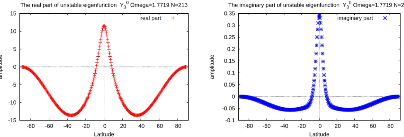
On the other hand, when Ω > 0, the eigenvalues converge fairly well. We find that the positive critical rotation rate Ω+c is 1.77194, and the critical azimuthal wavenumber mc = 2. Figure 2.4 shows the eigenvalues around Ω = Ω+B. The eigenvalues can be obtained with 0.1% accuracy when the truncation wavenumber is increased up to 63. The slightly unstable eigenfunction at Ω = 1.7719 is shown in figure 2.5. Obviously, no critical point is found, in contrast to the cases near the negative critical rotation rate.
2.4.2 Stability analysis with a shooting method
In the previous subsection, it is shown that in the spectral method ci does not converge even when the truncation wavenumber is increased, because the critical layers appear in the eigenfunctions. In this subsection, instead of the spectral method, we make use of a shooting method to overcome the difficulty.
2.4 Re-examination of the stability of inviscid zonal flow
-80 -60 -40 -20 0 20 40 60 80
-60 -40 -20 0 20 40 60
latitude
amplitude
The vorticity of unstable eigenfunction of Y30 Omega=-5.35 N=213
real part imaginary part
-80 -60 -40 -20 0 20 40 60 80
-80 -60 -40 -20 0 20 40 60 80
latitude
amplitude
The vorticity of the unstable eigenfunction of Y30 mc=1 Omega=-5.35
real part imaginary part
Figure 2.3: The vorticity of unstable eigenfunctions in the case of 3-jet zonal flow at Ω = Ω−B with azimuthal wavenumber m = 1: the left and right figures are obtained by the spectral method with truncation wavenumber N = 213 and by the shooting method, respectively.
0 0.005 0.01 0.015 0.02
20 40 60 80 100 120 140 160 180 200 ci
truncation wave number The imaginary part of phase angular velocity
around the critical rotation rate of Baines
Omega=1.76 Omega=1.77 Omega=1.75
-0.375 -0.37 -0.365 -0.36 -0.355 -0.35 -0.345
20 40 60 80 100 120 140 160 180 200 cr
truncation wave number The real part of phase angular velocity around the critical rotation rate of Baines
Omega=1.76 Omega=1.77 Omega=1.75
Figure 2.4: Same as figure 2.2 but for the unstable eigenvalues around Ω = Ω+B: the left and right figures show the imaginary part and the real part respectively.
-15 -10 -5 0 5 10 15
-80 -60 -40 -20 0 20 40 60 80
amplitude
Latitude
The real part of unstable eigenfunction Y30 Omega=1.7719 N=213 real part
-0.1 -0.05 0 0.05 0.1 0.15 0.2 0.25 0.3 0.35
-80 -60 -40 -20 0 20 40 60 80
amplitude
Latitude
The imaginary part of unstable eigenfunction Y30 Omega=1.7719 N=213 imaginary part
Figure 2.5: Same as figure 2.3 but for the vorticity of unstable eigenfunctions of 3-jet zonal flowY30 at Ω = 1.7719 with azimuthal wavenumberm = 2 with the truncation wavenumber N = 213: the left and right figures shows the imaginary part and the real part, respectively.
Equation (2.3) is expressed in the normal form as follows:
d dµ
( ψˆ φˆ
)
=
0 1
− l(l+ 1)U(µ) + 2Ω
{U(µ)−c}(1−µ2)+ m2 (1−µ2)2
2µ 1−µ2
( ψˆ φˆ
)
, (2.12)
where ˆφ=dψ/dµ.ˆ
For a given value of Ω, we obtain the solution ˆψ−and ˆφ− by integrating the normal form of the equation (2.12) from the edge pointµ=−1 to a certain pointµ0 ∈(−1,1) with the boundary conditions (2.4). Then we obtain the other solution ˆψ+ and ˆφ+ by integrating it from µ= 1 toµ=µ0.
The matching condition consists of continuity of streamfunction ˆψand its derivative φ, which is expressed byˆ
f(Ω, cr, ci) =
ψˆ+(µ0) ψˆ−(µ0) φˆ+(µ0) φˆ−(µ0)
= 0.
The point µ0 can be chosen at any point on the integral path. However, in this problem, the critical points are expected to exist around both the polesµ=±1. We then select µ0 as the end point of each integration and take µ0 = 0.1 which is far from both the poles.
In the above integrations, we should consider the singular points µ = ±1 and critical points µc such that U(µc)−c= 0.
First, in order to avoid the difficulty arising from the singular points, we change the starting point of the numerical integration from µ=±1 to certain nearby points. The values of ˆψ and ˆφ are obtained by using a power series expansion of the solution: At the
2.4 Re-examination of the stability of inviscid zonal flow south poleµ=−1, ˆψ is expanded into a power series of z =µ+ 1 as
ψˆ=zm/2 (
1 +
Jt
∑
j=1
ajzj )
(2.13) whereJtis a sufficiently large number and is taken up to 20. The coefficients aj of the series are successively determined by expanding (2.3) around µ= −1. The starting point should be close to the south pole to keep the accuracy of the power series expansion. Moreover, near marginal stability, the critical layer approaches the pole, which means that the convergence radius becomes small, and therefore we have to pay attention to the choice of the starting point. The same scenario holds also for the north pole. Second, we have to solve the singular behavior of the solution around the critical point µ=µc. Near marginal stability, the critical point approaches the interval [−1,1], and the numerical integration along the µ-axis rapidly becomes difficult. Then, in order to find the marginal stability eigenvalue as the limit of unstable eigenvalues, we deform the integral path in the complex µ-plane to bypass the critical points in such a way that π≤ argµ≤2π or 0 ≤argµ≤ π if U0(µc)>0 orU0(µc)<0, respectively.
Specifically, we employ a piecewise linear path as shown in figure 2.6. On integrating the normal form (2.12) from the south pole (A)µ=−1 to (E) µ0, we divide the integration path into four sections: (A)→(B)→(C)→(D)→(E), where the power series expansion is employed for the section (A)→(B), and the integrals for the other sections are performed by the 4th-order Runge-Kutta method with the number of grid points being about 3×10⁴. From the north pole (I) µ = 1 to (E), we perform the calculation in a similar way to the above in the order of (I)→(H)→(G)→(F)→(E).
We perform this shooting method to determinec=cr+ici for given values of Ω by use of the Newton method. The stopping condition of the Newton method is that the rate of the correction of the eigenvalues is less than 10−8. The Jacobi matrix
∂Re[f]
∂cr
∂Re[f]
∂ci
∂Im[f]
∂cr
∂Im[f]
∂ci
is evaluated by the central finite difference method with δcr, δci = 10−6.
We also perform this shooting method to determine Ωc andcrforci = 0. Skiba [31]
argued that numerical calculation of some eigenvalues is not stable because of the accumu- lation of the continuous spectrum. In our calculation we checked the numerical convergence of the eigenvalue by changing the number of grid points to 6×10³ and 6×10⁵ and confirmed that the relative errors ofcr and ci (or Ωc and cr) are less than 0.1%. Also, we have changed the increments of δcr and δci for the evaluation of the Jacobi matrix from 10−6 to 10−5 and found that the relative errors of the critical rotation rates and the eigenvalues remain less than 0.1%. Further, we have checked that the obtained eigenvalues and eigenfunctions are
Figure 2.6: Schematic of the integral path on the complex plane µ ∈ C. The solid and the dashed lines indicate the integrations by the expansion method and the Runge-Kutta method, respectively.
consistent with the inflection-point theorem and the semi-circle theorem, and that the ratio of the energy and the enstrophy of the eigenfunction is l(l+ 1) as derived by Skiba [32] for the zonal flow Yl0.
Figure 2.7 shows the stability eigenvalues obtained for the 3-jet zonal flow. For the sake of comparison, the eigenvalues obtained by the spectral method are also shown. It is seen that the eigenvalues obtained by the shooting method converge better than those obtained by the spectral method. We find the negative critical rotation rate Ω−c =−5.45685 and the critical azimuthal wavenumber mc = 1. The unstable eigenfunction at Ω = Ω−B is shown in figure 2.3 (right). The vorticity around the critical layers is more accurately shown in the shooting method solution, compared with the spectral method solution in figure 2.3 (left).
We also show the critical rotation rates of other zonal jet solutions (2.2) in table 3.2. There are a ∼ 10% differences between the critical rotation rates of Baines, Ω±B, and of the present study, Ω±c. When the number of zonal jets l is odd and Ω < 0, the critical layers emerge around both the north and the south poles. Whenl is even, the critical layer arises around the south (north) pole for Ω>0(<0). When l is odd and Ω>0, the critical eigenfunction does not have a singularity.
The inflection-point theorem states that when the basic flow is unstable, there is at least one zero point of ˜β= 2Ω +dYl0(µ)/dµ in the interval µ∈[−1,1]. This condition gives the possible range of the critical rotation rates, the upper and the lower bounds of which are given in table 3.2 as Ω±I. However, Ω±I do not coincide with Ω±c, with relative differences up
2.4 Re-examination of the stability of inviscid zonal flow
l-jet Ω±c m±c µ±c
Baines
Ω±B m±B relative
error Ω±I
relative difference
3 -5.4568 1 ±1 -5.35 1 1.95% −3√
7 45.4%
1.7719 2 - 1.76 2 0.673% 3√
7/4 11.9%
4 -9.7700 1 1 8.78 1 9.49% -15 53.5%
9.7700 1 -1 8.78 1 9.49% 15 53.5%
5 -19.22 1 ±1 -18.2 1 5.21% −15√
11/2 29.4%
4.022 3 - 3.90 3 3.03% −15√
11/16 177%
6 -28.389 1 1 -25.0 1 11.9% −21√
13/2 33.3%
28.389 1 -1 25.0 1 11.9% 21√
13/2 33.3%
7 -44.445 1 ±1 -40.0 1 10.0% −14√
15 24.2%
7.8929 3 - 7.226 3 8.44% 35√
15/32 86.3%
8 -59.618 1 1 -48.4 1 18.8% −18√
17 24.4%
59.618 1 -1 48.4 1 18.8% 18√
17 24.4%
9 -83.340 1 ±1 -69.3 1 16.8% −45√
19/2 17.6%
13.665 3 - 11.5 1 15.8% −315√
19/256 139%
Table 2.1: The critical rotation rates of inviscid zonal flows Ψ0 =−Yl0(µ)/l(l+ 1). Column 1 shows the number of jets l of the basic flows. Columns 2, 3, and 4 indicate the results of the present study: the critical rotation rate Ω±c , the critical azimuthal wavenumberm±c , and the sine latitude of critical layersµ±c. Columns 5, 6, and 7 are the results of [1] for the sake of comparison: the critical rotation rate Ω±B, the critical azimuthal wavenumberm±B, and the relative errors of critical rotation rates between [1] and the present study. Columns 8 and 9 indicate the critical rotation rates Ω±I estimated by the inflection-point theorem and their relative difference from the critical rotation rate Ω±c obtained by the present study.