Exact WKB analysis of second-order non-homogeneous linear ordinary differential
equations
By
Tatsuya KOIKE and Yoshitsugu TAKEI
September 2012
R ESEARCH I NSTITUTE FOR M ATHEMATICAL S CIENCES
KYOTO UNIVERSITY, Kyoto, Japan
Exact WKB analysis of second-order non-homogeneous linear ordinary differential
equations
By
Tatsuya Koike
∗and Yoshitsugu Takei
∗∗Abstract
In this paper we consider the exact WKB analysis of a second-order non-homogeneous linear ordinary differential equation with a large parameter. We give a geometric criterion which guarantees the Borel summability of formal solutions of a non-homogeneous equation;
this criterion is described in terms of exact steepest descent paths introduced in [AKT2]. An example related to the BNR equation ([BNR]) is also discussed from this viewpoint.
§1. Introduction and main result
In this paper we consider a second-order non-homogeneous linear ordinary differ- ential equation with a large parameter η (>0) of the following form:
(1.1)
d2
dx2 +ηp(x) d
dx +η2q(x)
ψ=F(x).
Here, for the sake of simplicity, we assume the coefficients p(x), q(x) and the non- homogeneous term F(x) are all polynomials of x. As (1.1) contains a large parameter η, we readily find that (1.1) has the following formal power series solution in η−1:
(1.2) ψ(x, η) =b
X∞
n=2
ψn(x)η−n,
Received ?, 200x, Accepted ??, 200x.
2000 Mathematics Subject Classification(s): 34M60, 34M30, 34E20
Key Words: exact WKB analysis, non-homogeneous equation, Borel summability, exact steepest descent path
Supported in part by JSPS grants-in-aid No.21740098, No.21340029 and No. S-24224001.
∗Department of Mathematics, Graduate School of Science, Kobe University, Kobe 657-8501, Japan.
∗∗Research Institute for Mathematical Sciences, Kyoto University, Kyoto 606-8502, Japan.
c
201X Research Institute for Mathematical Sciences, Kyoto University. All rights reserved.
where the coefficients ψn(x) (n= 2,3, . . .) are determined by the recursion formula
(1.3)
q(x)ψ2 =F(x), q(x)ψ3+p(x)dψ2 dx = 0, q(x)ψn+2+p(x)dψn+1
dx + d2ψn
dx2 = 0 (n≥2).
In general, the formal solution (1.2) does not converge. The purpose of this paper is to give a criterion that guarantees the Borel summability of the formal solution (1.2), that is, to discuss when the Borel sum
(1.4)
Z ∞ 0
e−yηψbB(x, y)dy
of ψ(x, η)b is well-defined, whereψbB(x, y) denotes the Borel transform of ψ(x, η), i.e.,b
(1.5) ψbB(x, y) :=
X∞
n=2
ψn(x)
(n−1)!yn−1.
Let us first explain the motivations of our research. In the case of a homogeneous equation
(1.6)
d2
dx2 +ηp(x) d
dx +η2q(x)
ψ = 0,
there exist the following formal solutions with an exponential term called WKB solu- tions:
(1.7) ψ±(x, η) = exp
η Z x
ζ±(x)dx X∞
n=0
ψ±,n(x)η−(n+1/2), where ζ±(x) are roots of the characteristic equation
(1.8) ζ2+p(x)ζ +q(x) = 0.
A criterion for the Borel summability of WKB solutions (1.7) is now well-known (cf.
[DLS], [CDK], [KS], etc.), as described in the following
Theorem 1.1. The WKB solutionsψ±(x, η) of the homogeneous equation (1.6) are Borel summable except on Stokes curves of (1.6). Here a Stokes curve of (1.6) is, by definition, an integral curve of the direction field
(1.9) Im (ζ+(x)−ζ−(x))dx= 0
emanating from a turning point of (1.6), i.e., a zero of the discriminant of (1.8). To be more precise, if the steepest descent paths of
(1.10) Re
± Z x
(ζ+(x)−ζ−(x))dx
passing through x0 can be prolonged to x = ∞ without flowing into any turning point, then the WKB solutionsψ±(x, η)normalized atx0are Borel summable in a neighborhood of x0.
One of our motivations is to generalize Theorem 1.1 to non-homogeneous equations.
As a matter of fact, since a general solution of (1.1) is given by a linear combination of the formal solution (1.2) and WKB solutions of (1.6), it suffices to consider only (1.2) to discuss the Borel summability of a general solution of (1.1) in view of Theorem 1.1.
Another motivation is concerned with generalization of Theorem 1.1 to third-order (or, more generally, higher-order) homogeneous equations. As is rigorously discussed in [KS], Theorem 1.1 can be proved by considering the Riccati equation (i.e., a first-order nonlinear ordinary differential equation) associated with (1.6) instead of dealing directly with (1.6). A crucial step in the proof is to apply the iteration method (or, equivalently, the fixed point theorem for a contraction mapping) after recursively solving first-order non-homogeneous linear ordinary differential equations which are, roughly speaking, obtained as linearized equation of the Riccati equation. Thus, in order to generalize this scheme to third-order homogeneous equations, we are compelled to solve a second- order non-homogeneous linear differential equation. As the first step toward the proof of the Borel summability of WKB solutions of higher-order equations, we investigate second-order non-homogeneous linear differential equations in this paper.
We now state our main result. Letx0 be a point that is not located on any Stokes curve of (1.6). Defining f±(x) by
f±(x) =− Z x
x0
ζ∓dx= 1 2
Z x x0
{−(ζ++ζ−)±(ζ+−ζ−)}dx (1.11)
= 1 2
Z x x0
{p(x)±(ζ+−ζ−)}dx,
we let Γ(0)± denote a steepest descent path of Ref± passing through x0. If Γ(0)+ (resp., Γ(0)− ) crosses a Stokes curve of (1.6) of type + > − (resp., of type − > +, where a Stokes curve of (1.6) is said to be of type + >− if Re Rx
(ζ+(x)−ζ−(x))dx >0 holds on the curve in question) at some pointx=x1, then we also consider a steepest descent path (“bifurcated steepest descent path”) Γ(1)− of Re f− (resp., Γ(1)+ of Ref+) passing through x1. In case these steepest descent paths Γ(0)± and Γ(1)± further cross a Stokes curve of (1.6), we similarly define Γ(2)± , Γ(3)± , . . . by repeating the same process. We now assume that these processes terminate in finite steps, that is, there exists a finite number of steepest descent paths{Γ(l)±}0≤l≤L so that every bifurcated steepest descent path passing through a crossing point of Γ(l)± and a Stokes curve of (1.6) is contained in {Γ(l)± }0≤l≤L. The totality of the steepest descent paths {Γ(l)± }0≤l≤L is called an “exact steepest descent path” of (1.1) passing throughx0. Under these situations we can prove
Theorem 1.2. The formal solution ψ(x, η)b of (1.1) of the form (1.2) is Borel summable at x = x0 if all the steepest descent paths belonging to an exact steepest descent path passing through x0 can be prolonged to x = ∞ without flowing into any turning point.
Note that exact steepest descent paths were first introduced in [AKT2] in the study of WKB solutions of homogeneous equations through the Laplace transformation method with respect to an independent variable of the differential equation (“exact steepest descent method”).
The paper is organized as follows: Making use of WKB solutions of the correspond- ing homogeneous equation (1.6) together with the method of variation of constants, we obtain an integral representation for the Borel transform of the formal solution ψ(x, η)b of (1.1) in Section 2. Then in Section 3 we study the analytic continuation of the Borel transform of ψ(x, η) by using this integral representation to prove Theorem 1.2.b In [AKT2] an exact steepest descent path was introduced to investigate the (inverse) Laplace integral for the Laplace transformed (with respect to an independent variable of the differential equation) WKB solutions. Here the integral representation obtained in Section 2 plays the same role as the (inverse) Laplace integral in [AKT2]; this explains why an exact steepest descent path appears in describing the condition for the Borel summability of ψ(x, η). Finally in Section 4 we discuss an example related to the BNRb equation, a third-order homogeneous equation for which a new Stokes curve appears, as was first observed by Berk et al ([BNR]).
§2. Explicit formula for the Borel transform of ψ(x, η)b
In this section, applying the method of variation of constants, we obtain an integral representation for the Borel transform ofψ(x, η) in terms of the Borel transform of WKBb solutions of the corresponding homogeneous equation (1.6).
Let
(2.1) ψ±(x, η) = exp
η Z x
x0
ζ±(x)dx
ϕ±(x, η), ϕ±(x, η) = X∞
n=0
ψ±,n(x)η−(n+1/2) be WKB solutions of the homogeneous equation (1.6) normalized at x0, where ζ±(x) are roots of (1.8). Note that ψ±(x, η) can be constructed by using formal power series solutions
(2.2) S±(x, η) =ηζ±(x) +S±,0(x) +η−1S±,1(x) +· · · of the Riccati equation
(2.3) S2+ dS
dx +ηp(x)S+η2q(x) = 0
associated with (1.6) in such a way that (2.4) ψ±(x, η) = 1
√Sodd
exp
−1 2η
Z x x0
p(x)dx± Z x
x0
Sodddx
, where Sodd denotes the odd part of S±(x, η), i.e.,
(2.5) S±(x, η) =±Sodd(x, η) +Seven(x, η).
For WKB solutions ψ±(x, η) we have
Lemma 2.1. Let W = W(ψ+, ψ−) = ψ+(dψ−/dx)−(dψ+/dx)ψ− denote the Wronskian of ψ+ and ψ−. Then the following holds:
(2.6) W(ψ+, ψ−) =−2 exp
−η Z x
x0
p(x)dx
.
Proof. Substituting (2.5) into the Riccati equation (2.3) and taking its odd part, we find
(2.7) 2SoddSeven+ dSodd
dx +ηp(x)Sodd = 0, that is,
(2.8) Seven =−1
2 d
dxlogSodd− 1 2ηp(x).
Note that (2.8) and a well known relation ψ± = exp Z x
S±dx justify the expression (2.4). Then, using the relation
(2.9) W(ψ+, ψ−) = d dx
ψ− ψ+
·ψ+2 =−2Soddexp
−2 Z x
x0
Sodddx
ψ+2 and (2.4), we immediately obtain
(2.10) W(ψ+, ψ−) =−2 exp
−η Z x
x0
p(x)dx
. This completes the proof of Lemma 2.1.
Using ψ± as a fundamental system of solutions of the corresponding homogeneous equation (1.6), we now apply the method of variation of constants to obtain a solution of the non-homogeneous equation (1.1). In view of Lemma 2.1, it is explicitly given by the following
1
2ψ+(x, η) Z x
F(x′) exp η
Z x′ x0
p(z)dz
ψ−(x′, η)dx′ (2.11)
− 1
2ψ−(x, η) Z x
F(x′) exp η
Z x′ x0
p(z)dz
ψ+(x′, η)dx′.
As the behavior of the first term is similar to that of the second term, we mainly consider only the second term of (2.11) in what follows. Furthermore, since the Borel summability of ψ± (or, more precisely, of ϕ±) is now known thanks to Theorem 1.1, we are going to discuss only the core part of the second term defined by the following, which will be denoted by Φ(x, η):
Φ(x, η) = exp η
Z x x0
ζ−(z)dz Z x exp
η Z x′
x0
(p(z) +ζ+(z))dz
F(x′)ϕ+(x′, η)dx′ (2.12)
= Z x
exp
−η Z x′
x
ζ−(z)dz
φ+(x′, η)dx′, where φ+(x′, η) =F(x′)ϕ+(x′, η).
We thus obtain a solution of the non-homogeneous equation (1.1) provided by (2.11). It can be expanded into the formal power series of η−1 as follows:
Proposition 2.2. The integral (2.12) is expanded as
(2.13) Φ(x, η) =
X∞
n=0
Φn(x)η−(n+3/2), the right-hand side of which is explicitly given by the following:
(2.14) −
X∞
n=0
η−(n+1) 1
ζ−(x′) d dx′
n 1
ζ−(x′)φ+(x′, η)x′=x.
Consequently (2.11)provides the formal power series solution (1.2) of (1.1) under con- sideration.
Proof. By a change of integration variable X′ =− Z x′
x
ζ−(z)dz, we have
(2.15) Φ(x, η) = Z 0
eηX′φe+(X′, η)dX′ with φe+(X′, η) =φ+(x′(X′), η)dX′ dx′
−1
. Then integration by parts tells us that
(2.16) Φ(x, η) =η−1eηX′φe+(X′, η)
X′=0− Z 0
η−1eηX′dφe+ dX′dX′. Using integration by parts repeatedly, we thus obtain
(2.17) Φ(x, η) =
X∞
n=0
(−1)nη−(n+1) d
dX′ n
φe+ X′=0
,
which verifies (2.14).
Thanks to Proposition 2.2 the formal power series solution (1.2) in question has an integral representation (2.11). In what follows we discuss the Borel summability of (2.11), mainly that of Φ(x, η) given by (2.12). To this end we first seek for an integral representation of the Borel transform of Φ(x, η), which is given by the following:
Proposition 2.3. The Borel transform of Φ(x, η), that is, the formal inverse Laplace transform of Φ(x, η) defined by
(2.18) ΦB(x, y) =L−1η→yΦ = X∞
n=0
Φn(x)
Γ(n+ 3/2)yn+1/2, has the following integral representation
(2.19) ΦB(x, y) =−
Z x∗
x
φ+,B(x′, y′(x′))dx′.
Here φ+,B(x, y) denotes the Borel transform of φ+(x, η), y′(x′) is a function defined by (2.20) y′(x′) =y+f+(x′) with f+(x′) =−
Z x′ x
ζ−(z)dz,
x∗ is a point determined byf+(x∗) =−y(i.e., y′(x∗) = 0), and the integral is performed along a path f+(x′) = −u (0 ≤ u ≤ y), i.e., along the steepest descent path of Ref+ passing through x.
Proof. It follows from (2.14) or, more conveniently, the equivalent expression (2.17) of Φ(x, η) that
(2.21) ΦB(x, y) = X∞
n=0
(−1)n yn Γ(n+ 1) ∗
d dX′
n
φe+,B
X′=0
,
where ∗ stands for the convolution product with respect to the variable y. Hence we have
ΦB(x, y) = X∞
n=0
(−1)n n!
Z y 0
(y−t)n d
dX′ n
φe+,B
X′=0
dt (2.22)
= Z y
0
φe+,B(t−y, t)dt
= Z 0
−y
φe+,B(X′, y+X′)dX′
= Z x
x∗
φ+,B x′, y− Z x′
x
ζ−(z)dz
! dx′.
This implies (2.19), completing the proof of Proposition 2.3.
Using Proposition 2.3, we investigate the analytic continuation of ΦB(x, y) to obtain the Borel summability of Φ(x, η) in the subsequent section.
§3. Proof of the main result (Theorem 1.2)
Assume that the point x0 in question is not located on any Stokes curve of the corresponding homogeneous equation (1.6). In what follows we show that the Borel transform ΦB(x0, y) of Φ(x0, η) given by the integral (2.19) can be analytically continued along the positive real axis {y ∈C|y≥0} under the condition of Theorem 1.2.
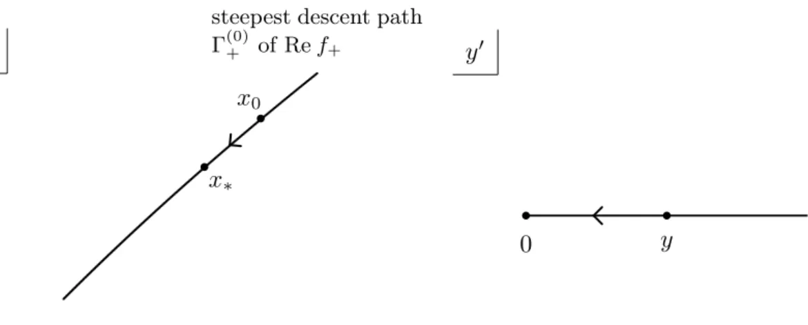
First of all, in view of the expression (2.19) and the analytic structure of φ+,B(x′, y′(x′)) near (x′, y′) = (x0,0), we can readily confirm that ΦB(x0, y) defines an ana- lytic function of y when |y| is small. (Cf. Figure 1. Note that, replacing the integral
x′
x0
x∗
steepest descent path Γ(0)+ of Ref+ y′
0 y
Figure 1. Integration path for ΦB(x0, y) when |y| is small.
(2.19) by a contour integral around x∗, we find that the square-root type singularity of φ+,B(x′, y′(x′)) at (x′, y′) = (x0,0) is irrelevant to the analyticity of ΦB(x0, y).) Thus our task is to verify the analytic continuability of ΦB(x0, y) wheny ≥0 is large. A key lemma is the following Lemma 3.1, which explicitly describes the singularity structure of the integrand φ+,B of (2.19).
Lemma 3.1. (i) The Borel transform φ+,B(x′, y′) =F(x′)ϕ+,B(x′, y′) of φ+(x′, η) =F(x′)ϕ+(x′, η) has a singular point at
(3.1) y′ =ω(x′) :=
Z x′ a
(ζ+(z)−ζ−(z))dz,
where a is a turning point of (1.6).
(ii) At y′ =ω(x′), φ+,B(x′, y′) satisfies the following relation:
(3.2) ∆y′=ω(x′)φ+,B(x′, y′) =iφ−,B(x′, y′−ω(x′)),
where ∆y′=ω(x′)φ+,B(x′, y′) denotes the discontinuity of φ+,B(x′, y′) at y′ =ω(x′), that is, the difference of the boundary value of φ+,B(x′, y′) from the upper side of the cut {y′ ∈C|Re (y′−ω(x′))≥0, Im (y′−ω(x′)) = 0} and the boundary value from its lower side.
It is a well known fact in the exact WKB analysis of second-order homogeneous ordinary differential equations that ϕ+,B(x′, y′) has the same singularity structure as described in Lemma 3.1 (see, e.g., [DP], [KT]). Since F(x) is a polynomial, Lemma 3.1 immediately follows from this fact.
It follows from Lemma 3.1 that the integrand of (2.19) is singular at a point where (3.3) y′(x′) =y−
Z x′ x0
ζ−(z)dz and y′(x′) = Z x′
a
(ζ+(z)−ζ−(z))dz
are satisfied. Eliminating y′(x′) in (3.3), we readily find that at a singular point of the integrand of (2.19) we have
(3.4) y−
Z x′ x0
ζ−(z)dz = Z x′
a
(ζ+(z)−ζ−(z))dz.
Since the left-hand side of (3.4) is real and positive for positivey, the integrand of (2.19) cannot have a singularity for positivey as far as the steepest descent path Γ(0)+ of Ref+
passing throughx0 is prolonged without flowing into any turning point or crossing any Stokes curve of (1.6). Hence ΦB(x0, y) is analytic along R+
y = {y ∈ C|y ≥ 0} under such a situation. On the contrary, if Γ(0)+ flows into a turning point, then ΦB(x0, y) has a singularity onR+
y in general as a singular point (3.1) hits the endpoint of the integral (2.19) at a turning point.
Now let us consider a more intriguing situation, that is, the situation where Γ(0)+ crosses a Stokes curve of (1.6) of type + > −. In this situation a singular point of the integrand φ+,B(x′, y′(x′)) hits a path of integration of (2.19) and consequently it becomes necessary to take the effect of such a singular point into acccount for sufficiently largey ≥0. For the sake of simplicity we suppose that the steepest descent path Γ(0)+ of Ref+ passing throughx0 crosses just one Stokes curve of type +>− emanating from a turning point a of (1.6) in what follows. We denote the crossing point of Γ(0)+ and the Stokes curve by x = x1. Then (3.4) implies that a singular point of the integrand φ+,B(x′, y′(x′)) hits a path of integration of (2.19) at
(3.5) y = ˆy :=
Z x1
a
(ζ+(z)−ζ−(z))dz+ Z x1
x0
ζ−(z)dz >0.
To analyze explicitly the effect of the singular point of φ+,B(x′, y′(x′)) to the analytic continuation of ΦB(x0, y) when y ≥ y, we first make a change of integration variableˆ from x′ to y′ =y+f+(x′) in (2.19) as follows:
(3.6) ΦB(x0, y) = Z 0
y
φ+,B(g+(y′−y), y′) dy′
ζ−(g+(y′−y)),
whereg+(y′) denotes an inverse function off+(x′), i.e.,y′ =y+f+(x′) can be expressed also as x′ =g+(y′−y). Rewriting (3.4) as
(3.7)
Z x′ x1
ζ+(z)dz=y− Z x1
a
(ζ+(z)−ζ−(z))dz− Z x1
x0
ζ−(z)dz =y−yˆ
and denoting x′ that satisfies (3.7) by x∗∗, we find that the integrand of (3.6) has a singularity at
(3.8) y∗∗:=
Z x1
a
(ζ+(z)−ζ−(z))dz+ Z x∗∗
x1
(ζ+(z)−ζ−(z))dz
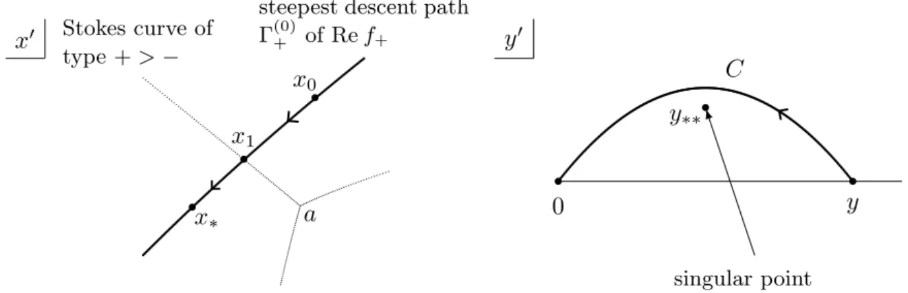
and the analytic continuation of ΦB(x0, y) to y ≥ yˆ is given by an integral of (3.6) along a path C indicated as in Figure 2. (Here we assume that Imy∗∗ > 0 for the
x′
a x0
x1
x∗
steepest descent path Γ(0)+ of Ref+
Stokes curve of type +>−
y′
▼
0 y
y∗∗
C
singular point of φ+,B
Figure 2. Integration path of (3.6) when y≥y.ˆ
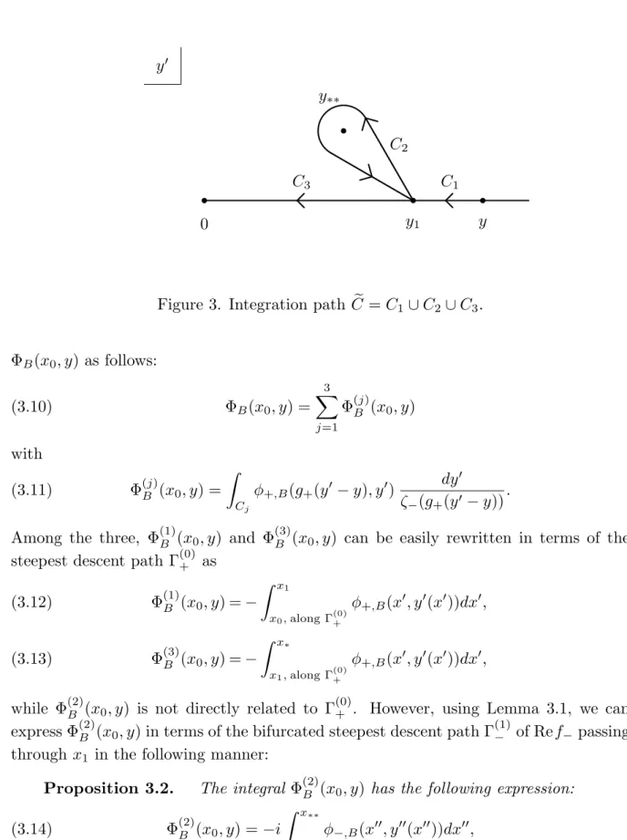
sake of definiteness.) Then we deform the path C to a new integration path Ce which is homotopically equivalent to C and consists of the following three portions:
(3.9) C ≃Ce =C1∪C2∪C3,
where
C1 : a path from y to y1 :=y′(x1) =y−Rx1
x0 ζ−dz on the real axis,
C2 : a path starting from y1, encirclingy∗∗ anticlockwise and returning to y1, C3 : a path from y1 to 0 on the real axis.
(Cf. Figure 3.) Corresponding to this decomposition of Ce ≃ C, we also decompose
y′
0 y1 y
y∗∗
C1 C3
C2
Figure 3. Integration path Ce=C1∪C2∪C3.
ΦB(x0, y) as follows:
(3.10) ΦB(x0, y) =
X3
j=1
Φ(j)B (x0, y) with
(3.11) Φ(j)B (x0, y) = Z
Cj
φ+,B(g+(y′−y), y′) dy′
ζ−(g+(y′−y)).
Among the three, Φ(1)B (x0, y) and Φ(3)B (x0, y) can be easily rewritten in terms of the steepest descent path Γ(0)+ as
Φ(1)B (x0, y) =− Z x1
x0,along Γ(0)+
φ+,B(x′, y′(x′))dx′, (3.12)
Φ(3)B (x0, y) =− Z x∗
x1,along Γ(0)+
φ+,B(x′, y′(x′))dx′, (3.13)
while Φ(2)B (x0, y) is not directly related to Γ(0)+ . However, using Lemma 3.1, we can express Φ(2)B (x0, y) in terms of the bifurcated steepest descent path Γ(1)− of Ref− passing through x1 in the following manner:
Proposition 3.2. The integral Φ(2)B (x0, y) has the following expression:
(3.14) Φ(2)B (x0, y) =−i Z x∗∗
x1
φ−,B(x′′, y′′(x′′))dx′′,
where y′′(x′′) is defined by
(3.15) y′′(x′′) = (y−y) +ˆ f−(x′′) =
y− Z x1
a
(ζ+−ζ−)dz− Z x1
x0
ζ−dz
+f−(x′′) with
(3.16) f−(x′′) =−
Z x′′
x1
ζ+(z)dz,
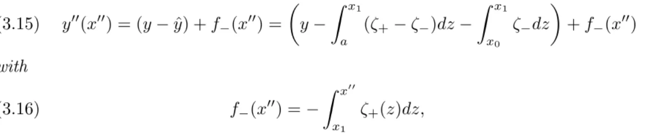
x∗∗ is a point determined by f−(x∗∗) =−(y−y) (i.e.,ˆ y′′(x∗∗) = 0, cf. (3.7)), and the integral is performed along a path f−(x′′) =−v (0≤v≤y−y), i.e., along the steepestˆ descent path of Ref− passing through x1 (cf. Figure 4).
x′′
a x0
x1
x∗
x∗∗
steepest descent path Γ(1)− of Ref−
Figure 4. Integration path of (3.14).
Proof. It follows from Lemma 3.1, (ii) that Φ(2)B (x0, y) =
Z
C2
φ+,B(g+(y′−y), y′) dy′ ζ−(g+(y′−y)) (3.17)
=− Z y1
y∗∗
∆y′=y∗∗φ+,B(g+(y′−y), y′) dy′ ζ−(g+(y′−y))
=−i Z y1
y∗∗
φ−,B(g+(y′−y), y′−ω(g+(y′−y))) dy′
ζ−(g+(y′−y)). Here, letting x′′ denote g+(y′−y), we employ a change of integration variable from y′ to y′′ =y′−ω(g+(y′−y)). Firstly, we note that x′′ =g+(y′−y) means
(3.18) y′−y =f+(x′′) =− Z x′′
x0
ζ−dz
and that
(3.19) y′′−y′ =−
Z g+(y′−y) a
(ζ+−ζ−)dz=− Z x′′
a
(ζ+−ζ−)dz holds. Hence
y′′ =y− Z x′′
x0
ζ−dz− Z x′′
a
(ζ+−ζ−)dz (3.20)
=y−
Z x1
x0
ζ−dz+ Z x1
a
(ζ+−ζ−)dz+ Z x′′
x1
ζ+dz
!
= (y−y) +ˆ f−(x′′).
Secondly, we have
dy′′ =dy′−(ζ+−ζ−)(x′′)dg+
dy′ (y′−y)dy′ (3.21)
=dy′−(ζ+−ζ−)(x′′) 1
(df+/dx)(x′′)dy′
=dy′+ (ζ+−ζ−)(x′′) ζ−(x′′) dy′
= ζ+(x′′) ζ−(x′′)dy′, that is,
(3.22) dy′′
ζ+(x′′) = dy′ ζ−(x′′).
Thirdly, it follows from the definition of x∗∗ and y∗∗ that x′′ =g+(y′−y) =x∗∗ holds when y′ = y∗∗ (cf. (3.4), (3.7) and (3.8)). Hence, by (3.8), we find that the point y′ =y∗∗ corresponds in the new variable y′′ to the point
(3.23) y′−
Z x′′
a
(ζ+−ζ−)dz y′=y
∗∗,x′′=x∗∗
= 0,
that is, y′′ = 0. On the other hand, since the definition of y1, i.e., y1 = y′(x1) = y +f+(x1) implies that g+(y1 −y) = x1, the point y′ = y1 corresponds in the new variable y′′ to the point
(3.24) y′− Z x′′
a
(ζ+−ζ−)dz y′=y
1,x′′=x1
=y− Z x1
x0
ζ−dz− Z x1
a
(ζ+−ζ−)dz=y−y.ˆ
We thus conclude
(3.25) Φ(2)B (x0, y) =−i Z y−yˆ
0
φ−,B(x′′, y′′) dy′′
ζ+(x′′) with y′′ = (y−y) +ˆ f−(x′′).
Finally, if we make a change of integration variable from y′′ to x′′ in (3.25), we obtain the expression (3.14) for Φ(2)B (x0, y).
Thanks to Proposition 3.2, each Φ(j)B (x0, y) (j = 1,2,3) has the same form as the original integral (2.19). Hence, if both the steepest descent paths Γ(0)+ and Γ(1)− are prolonged to x = ∞ without crossing any further Stokes curves of (1.6), the above reasoning verifies that each Φ(j)B (x0, y) (and hence ΦB(x0, y) as well) is analytically continued along the whole positive real axis. In case Γ(0)+ and/or Γ(1)− may cross any other Stokes curve of (1.6), we can apply the discussion in this section again to Φ(j)B (x0, y) as it has the same form as (2.19). Thus we obtain the analyticity of ΦB(x0, y) on the positive real axis {y∈C|y≥0} under the condition of Theorem 1.2.
Finally, the exponential growth of ΦB(x, y) with respect to the y-variable easily follows from that ofφ+,B(x, y) (cf. [KS]). The proof of Theorem 1.2 is now completed.
Remark. In case Γ(0)+ and Γ(1)− are prolonged to x = ∞ without crossing any further Stokes curves of (1.6), corresponding to the decomposition (3.10) of the Borel transform ΦB(x0, y), we can obtain the following expression of the Borel sum of Φ(x0, η) in view of Proposition 3.2:
(SΦ)(x0, η) = Z x0
x1,along Γ(0)+
exp
−η Z x′
x0
ζ−dz
(Sφ+)(x′, η)dx′ (3.26)
+ Z x1
∞,along Γ(0)+
exp
−η Z x′
x0
ζ−dz
(Sφ+)(x′, η)dx′
+i Z x1
∞,along Γ(1)−
exp
−ηyˆ−η Z x′′
x1
ζ+dz
(Sφ−)(x′′, η)dx′′, where SΦ denotes the Borel sum of Φ.
§4. An example related to the BNR equation
In [BNR] Berk et al considered the following third-order linear differential equation (4.1)
d3
dx3 + 3η2 d
dx + 2ixη3
ψ= 0
and showed that some Stokes phenomena for Borel resummed WKB solutions of (4.1) occur not only on ordinary Stokes curves but also on the so-called “new Stokes curves”.
Here an ordinary Stokes curve means a Stokes curve emanating from a turning point, while a new Stokes curve is a Stokes curve passing through no turning points. (See [AKT1] for more precise definitions of new Stokes curves.)
To be more concrete, as the characteristic equation of (4.1) is given by
(4.2) ζ3+ 3ζ+ 2ix= 0
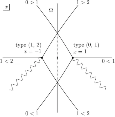
and a turning point is a zero of the discriminant of (4.2), i.e., a point where two characteristic roots merge, the BNR equation (4.1) has two turning points at x =±1, from each of which three Stokes curves emanate. See Figure 5 for the figure of Stokes curves of (4.1). In Figure 5 “a turning point of type (j, k)” means a turning point where two characteristic roots labeled by ζj and ζk merge. Similarly, “a Stokes curve of type j > k” is a Stokes curve on which Im Rx
(ζj(x)−ζk(x))dx = 0 and Re Rx
(ζj(x)− ζk(x))dx > 0 hold. (To number the characteristic roots, in Figure 5 we have placed two cuts, designated by wiggly lines, which enable us to define a characteristic root as a single-valued analytic function.) In addition to ordinary Stokes curves emanating from turning points new Stokes curves are also included in Figure 5: In the case of (4.1) the imaginary axis is a new Stokes curve. Note that, as is shown in [BNR] and [AKT1], Stokes phenomena for Borel resummed WKB solutions do really occur on the solid portion of the new Stokes curve, but not on its dashed portion.
Figure 5. Stokes curves of the BNR equation (4.1).
Here let us recall the construction of WKB solutions of (4.1). We first assume that
an unknown function ψ of (4.1) has the form
(4.3) ψ = exp
Z x
S(x, η)dx.
Then, substituting (4.3) into (4.1), we find that S(x, η) should satisfy
(4.4) S3+ 3SdS
dx + d2S
dx2 + 3η2S+ 2ixη3 = 0,
a higher-order analogue of the Riccati equation (2.3). Equation (4.4) has the following formal power series solution with the characteristic root ζj (j = 0,1,2) of (4.2) as its top order term:
(4.5) S(j)(x, η) =ηζj(x) +S0(j)(x) +η−1S1(j)(x) +· · · .
A WKB solution ψj(x, η) of (4.1) is a formal solution obtained by substituting (4.5) into (4.3).
We now set S =ηζ0(x) +T in (4.4). ThenT should satisfy
(4.6) d2T
dx2 + 3ηζ0(x)dT
dx + 3η2((ζ0(x))2+ 1)T +R= 0 with
(4.7) R= 3η2ζ0dζ0
dx +ηd2ζ0
dx2 + 3ηdζ0
dxT + 3ηζ0T2+T3+ 3TdT dx.
The remainder term R consists of terms containing only ζ0, lower order terms with respect toη, and higher order (i.e., nonlinear) terms with respect toT. In what follows, neglecting the remainder term R and regarding it as a given non-homogeneous term, we consider
(4.8)
d2
dx2 + 3ηζ0(x) d
dx + 3η2((ζ0(x))2+ 1)
T =F(x)
as an example of application of our main theorem (Theorem 1.2). Note that the ho- mogeneous equation corresponding to (4.8) is nothing but (the principal part of) the linearlized equation or the Fr´echet derivative of (4.4) at its formal solution S(0)(x, η).
Our main interest lies in the Borel summability of the formal solution (1.2) of (4.8) and its comparison with that of WKB solutions of the BNR equation (4.1).
Equation (4.8) can be written also in terms of ζj as (4.9)
d2
dx2 −η (ζ1−ζ0) + (ζ2−ζ0) d
dx +η2(ζ1−ζ0)(ζ2−ζ0)
T =F(x).
Hence the characteristic roots of (4.9) are given by
(4.10) ζ1−0 :=ζ1−ζ0 and ζ2−0 :=ζ2−ζ0
and (4.9) has only one turning point at x = −1. (The other turning point x = 1 is a kind of singular points in discussing (4.9).) We also set
(4.11) f1−0(x) =− Z x
x0
ζ2−0dx and f2−0(x) =− Z x
x0
ζ1−0dx.
From now on, applying Theorem 1.2, we investigate the Borel summability of the formal solution (1.2) of (4.8) (or equivalently (4.9)) when x0 lies in the region Ω specified in Figure 5 or its boundary.
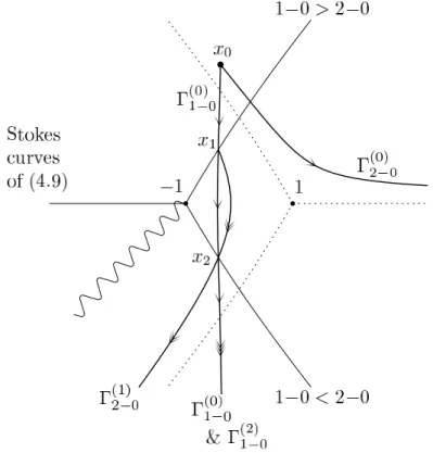
Case (I) (when x0 lies in the interior of Ω.)
When x0 lies in the interior of Ω, the configuration of the steepest descent paths Γ(0)1−0 of Ref1−0 and Γ(0)2−0 of Ref2−0 passing through x0 become as is indicated in Figure 6. While Γ(0)2−0 is prolonged tox=∞without crossing a Stokes curve of (4.9) of
Figure 6. Exact steepest descent path passing through x0 in Case (I).
type 2−0>1−0, Γ(0)1−0 crosses a Stokes curve of type 1−0>2−0 atx1. Thus we need to take into account also a bifurcated steepest descent path Γ(1)2−0 passing through x1. Since Γ(1)2−0 again crosses a Stokes curve of type 2−0>1−0 atx2, we should consider another bifurcated steepest descent path Γ(2)1−0, which coincides with the original Γ(0)1−0 (thanks to the symmetry of the equation with respect to the real axis) in this case.
As is clearly visualized in Figure 6, all the steepest descent paths Γ(0)1−0, Γ(0)2−0, Γ(1)2−0 and Γ(2)1−0 are prolonged to x=∞. Thus Theorem 1.2 guarantees the Borel summability of the formal solution (1.2) in this case.
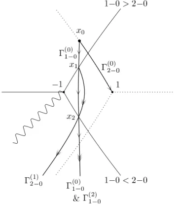
Case (II) (when x0 lies on the left boundary of Ω, i.e., on a Stokes curve of (4.1).) If we pick up a pointx0 from the left boundary of Ω, that is, from a Stokes curve of (4.1), then one of the steepest descent paths Γ(0)2−0 passing through x0 flows into x = 1 and cannot be prolonged to x =∞ (cf. Figure 7). Thus the Borel summability of the
Figure 7. Exact steepest descent path passing through x0 in Case (II).
formal solution (1.2) is not expected to hold in this case.
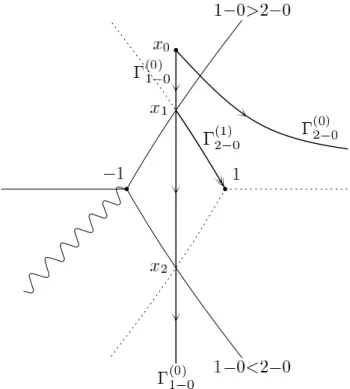
Case (III) (when x0 lies on the right boundary of Ω, i.e., on a new Stokes curve of (4.1).)
Finally we consider the case where x0 lies on the right boundary of Ω, that is, on a new Stokes curve of the BNR equation. In this case there is no problem with Γ(0)2−0, but the steepest descent path Γ(1)2−0 bifurcated from Γ(0)1−0 atx1 flows intox= 1 and cannot be prolonged to x = ∞, as is shown in Figure 8. Hence, similarly to Case (II) (but due to different geometric obstruction), the Borel summability of the formal solution (1.2) is not expected to hold in Case (III) as well. In this way the new Stokes curve of the BNR equation (4.1) is also captured through the analysis of the non-homogeneous
Figure 8. Exact steepest descent path passing through x0 in Case (III).
second-order equation (4.9).
References
[AKT1] Aoki, T., Kawai, T. and Takei, Y., New turning points in the exact WKB analysis for higher-order ordinary differential equations, Analyse alg´ebrique des perturbations singuli`eres. I, Hermann, Paris, 1994, pp. 69–84.
[AKT2] , On the exact steepest descent method: A new method for the description of Stokes curves,J. Math. Phys.,42(2001), 3691–3713.
[BNR] Berk, H. L., Nevins, W. M. and Roberts, K. V., New Stokes’ line in WKB theory, J.
Math. Phys.,23(1982), 988–1002.
[CDK] Costin, O., Dupaigne, L. and Kruskal, M. D., Borel summation of adiabatic invariants, Nonlinearity, 17(2004), 1509–1519.
[DP] Delabaere, E. and Pham, F., Resurgent methods in semi-classical asymptotics, Ann.
Inst. H. Poincar´e,71 (1999), 1–94.
[DLS] Dunster, T. M., Lutz, D. A. and Sch¨afke, R., Convergent Liouville-Green expansions for second-order linear differential equations, with an application to Bessel functions, Proc. Roy. Soc. London, Ser. A,440(1993), 37–54.
[KT] Kawai, T. and Takei, Y., Algebraic Analysis of Singular Perturbation Theory, Amer.
Math. Soc., 2005.
[KS] Koike, T. and Sch¨afke, R., On the Borel summability of WKB solutions of Schr¨odinger
equations with polynomial potentials and its applications, in preparation.