Ichimiya and Nakamura, Transactions of the JSME (in Japanese), Vol. 00, No. 00 (201x)
各種情報量と複雑度を用いた混合層の層流―乱流遷移過程の解析
(変動渦度と乱れエネルギー散逸率の解析)
一宮 昌司
*1,中村 育雄
*2Various information and complexity measures for analyzing the laminar-turbulent transition
process in mixing layer
(Analysis of fluctuating vorticity and turbulent energy dissipation rate)
Masashi ICHIMIYA
*1and Ikuo NAKAMURA
*2*1 Department of Mechanical Science, Tokushima University 2-1 Minami-Josanjima-cho, Tokushima-shi, Tokushima 770-8506, Japan
*2 Emeritus Professor, Nagoya University Furo-cho, Chikusa-ku, Nagoya-shi, Aichi 464-8601, Japan Received: XXXX; Revised: XXXX; Accepted: XXXX Abstract
In this paper, the laminar-turbulent transition process of a mixing layer downstream of a two-dimensional nozzle exit was analyzed based on various information and complexity measures. Shannon entropy, permutation entropy, and approximated Kolmogorov complexity were also obtained. To obtain the Shannon entropy, the temporal probability distribution of the hot-wire output voltage data was determined and analyzed. In addition to the fluctuating velocity, its time derivative and the square of this derivative were analyzed. The Shannon entropy of the time derivative and its square slightly decreased downstream, in accordance with the increase in the time scale of the turbulence. When the length of the extracted data was constant, the permutation entropy of the time derivative and its square increased around the peripheral region of the mixing layer, in accordance with the intermittent nature of the velocity signals. The region is at the 3-4 times farther from the jet centerline than the region where the fluctuating velocity becomes maximum. When the length of the extracted data was varied in accordance with the integral time scale of turbulence, the permutation entropy initially decreased in the potential core and subsequently increased after the disappearance of the potential core, as the transition progressed. The approximated Kolmogorov complexity of the time derivative and its square were smaller than that of the fluctuating velocity. Owing to the simplification of the data, they slowly increased after the disappearance of the potential core and then quickly decreased after the development of turbulence.
Keywords : Transition, Turbulence, Turbulent flow, Shannon entropy, Permutation entropy, Kolmogorov complexity,
Mixing layer
1. 緒 論
乱流の特性の重要な点は,その運動の不規則性にある.これは例えば,粘性流体力学の代表的な本の一つ (Schlichting and Gersten, 2000a)に記載されている"high irregular, random, fluctuating motion"に端的に表現されている. 秩序だった層流から,この不規則な乱流への遷移過程は流体力学の大きな問題であり,また工業上も表面摩擦, 流れの剥離に関連して重要である.遷移過程自身が複雑であることは,壁に沿う流れの遷移の系統を表現した Morkovin マップ(例えば Panton, 2005a)によく表現されている.
著者らはこれまでに,遷移過程の一つである自由せん断層の乱流遷移過程に関連して一連の研究を行ってきた が,そこでは壁面せん断流で使われるような乱れ強さの増加のような単調に変化する遷移移行の測度が,それま
No.20-00130 [DOI: 10.1299/transjsme.20-00130]
*1 正員,徳島大学大学院 社会産業理工学研究部(〒770-8506 徳島県徳島市南常三島町 2-1) *2 正員,名誉員,フェロー,名古屋大学名誉教授(〒464-8601 愛知県名古屋市千種区不老町) E-mail of corresponding author: [email protected]
Bulletin of the JSME Vol. 00, No. 00, 201x
日本機械学会論文集
でになされた研究では明らかではないことを認識し(一宮他,2011b)(Ichimiya et al., 2013),これを改善すべく乱流 遷移過程中の諸量の複雑さへの変化という特性に注目してコルモゴロフ複雑度(Kolmogorov, 1965, 1983)に基づく 解析を行い,その有効性を示した(一宮,中村,2012)(Ichimiya and Nakamura, 2013).そしてこれを,その後,壁面 せん断流乱流遷移過程にも適用した(一宮他,2014)(一宮他,2015).
次に,シャノンエントロピー(Shannon, 1948)(Shannon and Weaver, 1949)と,Bandt と Pompe(2002)の順列エントロ ピー(permutation entropy)を用いた熱線風速計瞬時波形データのディジタル化されたものの解析を行い(一宮,中 村,2017),変動速度の確率分布のシャノンエントロピーは,混合層の乱流遷移過程において単調に増加して,乱 流遷移の測度となり得ることを明らかにした.また,変動速度の順列エントロピーは下流に進むと,増加,減少, 再増加,再減少と変化するが,これは混合層の乱流遷移過程における変動速度の増加や,周期変動から不規則変 動への様式の変化を反映していることを解明にした.さらに,変動速度の確率密度関数の Kullback-Leibler のダイ バージェンスは,初めは増加するが,最大となった後は下流で減少して,混合層の乱流遷移過程を通して単調に は変化しないことを明らかにした.さらに,シャンノンエントロピーが乱流場で満たすべき方程式を導き,レイ ノルズ応力との関連など幾つかの考察を加えた.なお自由せん断流の遷移過程においては,管内流遷移の際に現 れる乱流パフやスラグ,あるいは壁面境界層の遷移に見られる乱流斑点のような局在化した乱流塊はこれまで報 告されていないが,後述の図 13 では斑点的な波形が見られる.しかしこの波形は壁面乱流で見られる遷移過程の 波形(Schlichting and Gersten, 2000b)とは異なっている.なお,このような乱流と非乱流の界面そのものの研究につ いては文献(Eames and Flor, 2011)(Hunt et al., 2011)(da Silva et al., 2014)などがある.
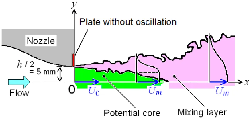
さて,乱流の特徴を表すものには,変動速度自体の他にも,変動渦度や乱れエネルギー散逸などもある.ゆえ にこれらの情報量解析を行って,それらの類似性や相違性を検討することは,情報量解析の有用性や問題点を理 解するのみならず,自由せん断流の乱流遷移過程の理解を深める一助にもなろう. そこで本研究は前報(一宮,中村,2017)の変動速度の解析をさらに進めて,変動渦度と乱れエネルギー散逸 の情報量解析や複雑度解析を行う.オーダー的にはこれら 2 量は,変動速度 u の時間微分係数とその 2 乗をそれ ぞれ調べることに相当するので,時間微分係数∂u/∂t や(∂u/∂t)2を解析する.後者は前者の 2 乗であるが,異なる物 理量であるので,それぞれ考察する.これらは時間に対する変化量であるので,シャノンエントロピーや順列エ ントロピーを,原物理量や乱流の時間スケールと共に考察する. 2. 実験装置及び実験方法 解析した流れは,静止流体中に噴出する噴流の初期に形成される混合層である.噴流は幅 310 mm,高さ h = 10 mm の 2 次元ノズル出口(流れ方向座標 x = 0)から噴出する.図 1 に流れ場の上半分及び座標系を示す.著者ら はこれまでこの流れの平均,変動速度分布,噴流の広がり,撹乱の運動エネルギーの生成率,対流率及び散逸率 の下流への変化などを調べた(一宮他,2011a)(Ichimiya et al., 2011).また乱流遷移過程の垂直方向への進行を明ら かにしたり,佐藤の雑然度(Sato and Saito, 1975)を求めて遷移進行への適用可能性を調べた(一宮他,2011b)(Ichimiya
Fig. 1 Schematic diagram of the two-dimensional mixing layer and coordinate system. The mixing layer is formed between the jet and the surrounding quiescent fluid.
et al., 2013).またノズル出口に制御された撹乱発生用として取り付けた振動板の振幅や周波数の影響(一宮他, 2013)を調べ,振動板の振動様式の影響(Ichimiya et al., 2014)を検討した.
本解析は,この流れのコルモゴロフ複雑度解析(一宮,中村,2012)(Ichimiya and Nakamura, 2013),シャノンエン トロピー解析や順列エントロピー解析(一宮,中村,2017)と同様に,ノズル出口に上下一枚ずつ設置した振動板が ノズル出口断面を狭めないように静止させた場合のみを対象とした.実験は,ノズル出口直後の速度 U0とノズル 出口高さ h に基づくレイノルズ数を 5000(U0 ≒ 7.5 m/s)として行なった.測定には各受感部直径 5 m,長さ l = 1 mm の X 型熱線プローブを用いた.風速に比例した熱線出力電圧はサンプリング周波数 5 kHz で 262144 個 (約 52 秒間)サンプリングされた.そのデータから合成された流れ方向変動速度 u に対応する電圧 e(分解能e = 0.002 V)とその時間微分係数∂e/∂t とその 2 乗(∂e/∂t)2を解析する.時間微分係数は,前後 2 点ずつの値を含む 5 点間を 2 次式近似して差分して求めた.このため∂e/∂t とその 2 乗(∂e/∂t)2のデータ数は e のそれよりも 4 個少ない 262140 である.なお,ここでは記号は実測の電圧 e を用いたが,物理的には記号 u を使う方が自然なので,以下 では u を用いる.空間分解能が X 型熱線プローブに及ぼす影響を Burattini(2008)に従って評価したところ,u の 2 乗平均 では真値に対する最大誤差は約 5%(最悪で真値の 95%に過小評価される),u の空間微分係数 2 乗平均 では真値に対する最大誤差は約 35%と評価された.このように特に微分係数には空間分解能が大きく影 響するが,本研究で求めるシャノンエントロピーと順列エントロピーは,一つの測定位置における 262140 個間の 最大値と最小値にわたる確率分布状況などを解析するので,得られる値は誤差にかかわらない.またコルモゴロ フ複雑度解析においては,位置による誤差の差異を考慮して考察を行う. 測定は垂直方向座標 y ≧ 0 の範囲で行った.測定は,ポテンシャルコアが消滅して混合層の自己保存が成立す る位置よりも十分下流の x/h = 25 まで行った. 3. データ解析手法 3・1 シャノンエントロピー シャノンエントロピーは,前報(一宮,中村,2017)と同様に自己情報量の期待値として次式で求めた.ここで対 数の底は 2 とした.この場合,単位[bit]がつけられる. i n i i p p log 1
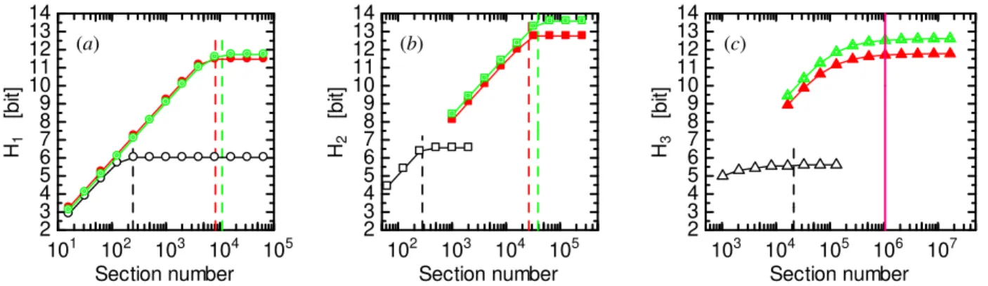
(1) ここで piは,離散確率空間上の確率分布 P が与えられたとき,n 個存在する各事象 Xiの確率 P(Xi)である.また pi = 0 のときは pi log pi = 0 と定義する.前報(一宮,中村,2017)で説明したように,シャノンエントロピーは不確か さの度合いを表すもので,これを前報の序論で引用した乱流場に適用した先行研究にならい,本研究はいまだ適 用例がない乱流遷移過程に用いた.ここで乱流中にも組織構造中ではこの秩序性を反映してシャノンエントロピ ーはむしろ小さくなることも予想されるので,その挙動の解釈には慎重な検討が必要である.なお前報では,同 じく確率分布に基づくモーメントとの差異にも言及している. 本研究におけるシャノンエントロピーは,前述のように流れ方向変動速度 u,その時間微分係数∂u/∂t 及びその 2 乗(∂u/∂t)2に対して確率を計算して求める.確率の計算を行なうためには,事象の 1 区間の幅を決定する必要が ある.区間幅が狭くなれば式(1)における区間数 n が増加し,一般に区間数が増加すればシャノンエントロピーは 増加するからである.そこで代表的な 3 位置(ノズル出口直後の中心線上の層流(x/h = 0.5, y/(h/2) = 0),流れ方 向時間平均速度からの変動速度の rms 値 u’が最大の位置 x / h = 8, y / (h/2) = 1.3 の乱流,及び十分下流の x / h = 20, y / (h/2) = 3.6 の乱流)において区間数に対するシャノンエントロピーH の変化を調べた.なお,これら 3 位置の 統計量の値は前報に示している(一宮,中村,2017).262144 個または 262140 個のデータの範囲(最大値と最小値 の差)をさまざまな分割数で分割したときの u,∂u/∂t,(∂u/∂t)2の H(それぞれ H 1,H2,H3と記す)の変化を図 2 に示す.u の場合(図2(a))は,初めは区間数の増加と共に H1は増加する.各位置の(umax– umin) / ∆u の値に縦破線を引 いたが,区間数がこれを越えると H1は一定値に飽和する.これは分解能以上に区間が細分化されて増えても,そ の区間内にはデータが存在しないから pi log pi = 0 となって H1に寄与しないからである.そこで,H1にはその飽 和値を採用することにした.これは前報(一宮,中村,2017)に述べたとおりである. 時間微分係数∂u/∂t の場合(図2(b))も,u の場合と同様に,初めは区間数の増加と共に H2は増加するが,区間 数が分解能(縦破線)を越えると H2は一定値に飽和する.そこで,H2にはその飽和値を採用した.この飽和する 分割数は,同じ測定位置の u のそれに比べると,約1~4 倍となった. 時間微分係数の2 乗 (∂u/∂t)2の場合(図2(c))も,初めは区間数の増加と共に H3は増加するが,乱流(緑三角 印,赤三角印)においては区間数をかなり多くしなければ H3の増加率は鈍らず,飽和する区間(x/h = 0.5, y/(h/2) = 0 では黒色縦破線,他の 2 位置では 108以上)まで数を増やし続けても,区間数が106を越えると計算時間が膨 大になるので,飽和していなくても区間数を1048577(分割数 1048576 = 220)(赤色縦実線)とし(∂u/∂t)2全データ を計算した.図2(c)より,分割数がそれより多くても H3はほぼ一定であるので,問題ないと判断される. 3・2 順列エントロピー シャノンエントロピーでは考慮されていないデータの順序に基づく大小関係を考慮して,Bandt と Pompe(2002) が提案した順列エントロピーを,本論文でも前報(一宮,中村,2017)と同様に求めた.要素 T 個の時系列(x1, x2,…, xT)から要素 n 個の数列(xt+1, xt+2,…, xt+n)を,0≦t≦(T– n) に亘って T – n +1 回取り出すとき,n 個要素内に相等しい 値がまったくなければ,大小関係の事象(順列)の数は n!である.このとき各順列の確率 piは,(0≦t≦(T – n)の 範囲内での,その順列の個数)/ (T – n +1)となるので,そのエントロピー(順列エントロピー)Hpがシャノンエ ントロピーと同様に, i n i p p p H log !
− = (2) で定義される.順列エントロピーを,n – 1 または log n!で正規化することもある. 順列エントロピーを求めるに当り,決定しておくべき条件については,前報と同様にまず n 個の要素内に相等 しい値が複数あるという事象も順列に含めた.次に,取り出す数列の要素数 n も前報と同様に8 とした.ただし, この要素数選択に関しては4・4 節で検討する.最後に元の時系列の要素数 T の選択であるが,これはサンプリ ングしたデータまたは微分係数が求められたデータをすべて用いた.すなわち u の場合は前報と同様に262144 で あり,∂u/∂t や(∂u/∂t)2では前述したように262140 である.Fig. 2 Shannon entropy as a function of section number: (a) fluctuating velocity, (b) time derivative of fluctuating velocity, and (c) square of the time derivative of fluctuating velocity. Black, x/h = 0.5, y/(h/2) = 0, laminar; green, x/h = 8, y/(h/2) = 1.3, turbulent; red, x/h = 20, y/(h/2) = 3.6, turbulent. Vertical broken lines correspond to the value of the difference between the maximum and minimum value of each position, divided by the data solution. Vertical solid red line in (c) indicates the section number used to calculate the Shannon entropies of the square of the time derivative of fluctuating velocity. Shannon entropies initially increase and then become constant.
102 103 104 105 2 3 4 5 6 7 8 9 10 11 12 Section number H2 [ b it] (b) 101 102 103 104 105 2 3 4 5 6 7 8 9 10 11 12 Section number H1 [ b it] (a) 103 104 105 106 107 2 3 4 5 6 7 8 9 10 11 12 Section number H3 [ b it] (c)
また,特に層流においては,信号中に存在する高周波ノイズのために値の差異が生じるので,この高周波ノイ ズを除去するために,前報と同様に,原データにそのデータの変動速度rms 値 u’を乗じることにより,u’が小さ い層流では変動がデータの分解能以下に減衰するようにさせた.具体的には,前述の変動最大位置 x/h = 8, y / (h/2)
= 1.3 では局所の u’を乗じても値が変わらないように,原データに (局所位置の u’ / U0)/(変動最大位置の u’ / U0)
を乗じた.
3・3 コルモゴロフ複雑度
本流れ場のコルモゴロフ複雑度解析は,著者らのこれまでの論文(一宮,中村,2012)(Ichimiya and Nakamura, 2013)(一宮他,2014)(一宮他,2015)で詳しく説明されてきたので,ここでは簡単に説明する.本論文では,実験デ ータ(熱線風速計出力をA/D 変換した離散データ列)を圧縮プログラムで調べ,その複雑度を,次式
AK(X) =𝐶(𝑋)|𝑋| (3)
のように,元データ X の長さ(データ容量)|X|に対する圧縮プログラムで圧縮された X の長さ C(X)の比で示され る近似コルモゴロフ複雑度AK で表示する.
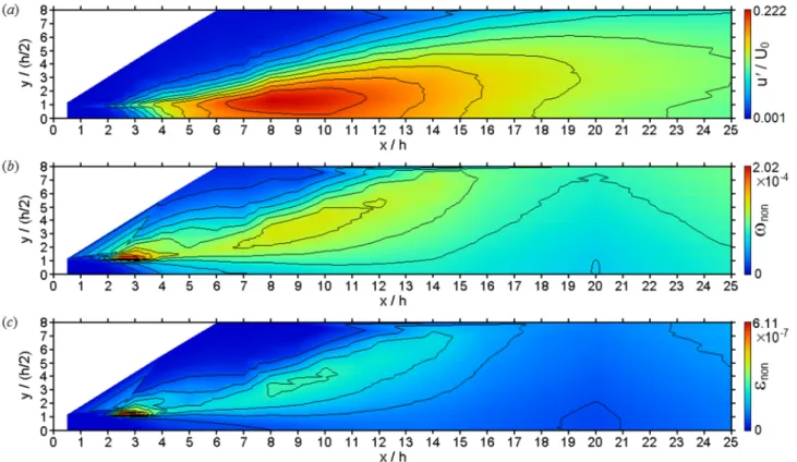
解析には既報(一宮,中村,2012)(Ichimiya and Nakamura, 2013)と同様に,0.2 ms おきにサンプリングされた流れ 方向変動速度 u を,32768 個(約 6.6 秒分)用いた.小数点や負号を除くために,各値から 32768 個内の最小値を 引き,ノズル出口直後速度 U0で無次元化した後,元の速度データが12 ビットすなわち 4096 分割されていること を考慮し,各データを000 から 999 までの 3 桁の整数に変換して,最後に横一列に並べた 98304 個の数値データ をテキストファイルに保存した.これによって分割数が4096 から 1000 に減少するが,その代わりデータ桁数が 12 から 3 に減少するので,同一データ内の桁間の値の変化が圧縮率に及ぼす影響を抑制できる.なお,桁数が変 化してもAK の分布形状は,全体として値が大きい方または小さい方に移動するだけであり,また例えば最大値 と最小値間の差は桁数によらずほぼ一定である(一宮他,2015).このデータを Windows パソコン上で圧縮した. 用いる圧縮形式は既報(一宮,中村,2012)(Ichimiya and Nakamura, 2013)で詳しく検討しており,これに基づいて 7z を用いた. 4. 解析結果及び考察 4・1 原物理量 本論文の主題である情報量解析や複雑度解析を行う前に,その元である原物理量の u や変動渦度ベクトルω の 大きさω = |ω |及び乱れエネルギー散逸率ε の空間分布を,本節ではまず示す.図 3(a)~(c)は u やω の 2 乗平均値 ω'及びε の x-y 平面上のコンター(すなわち,これらの量の等値線と色別による値の分布)を表したものである. ω は定義より, ω =
(
𝜕𝑤 𝜕𝑦−
𝜕𝑣𝜕𝑧,
𝜕𝑢𝜕𝑧−
𝜕𝑤𝜕𝑥,
𝜕𝑥𝜕𝑣−
𝜕𝑢𝜕𝑦) =
(𝜔𝑥, 𝜔𝑦, 𝜔𝑧) ∴ω = √𝜔𝑥2+ 𝜔𝑦2+ 𝜔𝑧2 ~√(
𝜕𝑢𝜕𝑦)
2 ∴ω' = √𝜔̅ ~ 2√(
𝜕𝑢 𝜕𝑦)
2̅
(4) と見積もられる.さらにRotta(1962)によれば,𝜕𝑢 𝜕𝑦
~
𝜕𝑢𝜕𝑥 と評価されるので, 𝜔′ ~√(
𝜕𝑢 𝜕𝑥)
2̅
~ 1 𝑈√(
̅
𝜕𝑢𝜕𝑡)
2 (5) と見積もられる.式(5)の右辺は次段落で述べる Taylor の凍結乱流仮説によって得られる.熱線風速計で変動速度 の空間微分を得るのが困難であるのに対し,上の評価によれば熱線データの時間微分により変動渦度の大きさの 空間変化などを知ることが可能となる. 一般に熱線風速計のデータは時系列データであり,これに基づいて乱流の空間構造を推測する必要がある.こ の方法として早くに提案されたのが,Taylor(1938)の凍結乱流仮説である.これは重要な仮説なので各著書で各種 の形で述べられている(Hinze, 1975)(Pope, 2000)(Panton, 2005b).その妥当性,補正などに関しても多くの研究があ り(Hinze, 1975),最近でも幾つかの研究がある(Tsinober et al., 2001)(Moin, 2009)(del Álamo and Jiménez, 2009)(He et al., 2010)(Higgins et al., 2012)(Geng et al., 2015)(Shet et al., 2017)(Yang and Howland, 2018).元来の Taylor の仮説は,ある空間測定点での乱れの時間的変化は,その時点での乱れの空間的パターンが一定のまま(凍結したまま),そ
の測定点を通過することから生ずると仮定するものである.Taylor はこれを,式 u = φ (t) = φ (x/U)が成立すること としている.Hinze(1975)では,次の偏微分の関係が成り立つこととしている.
𝜕
𝜕𝑡 = – U𝜕𝑥𝜕 (6)
Pope(2000)は‘flying hot wire’法による測定を例にとり説明している.また,格子乱流では Taylor の凍結乱流仮説 は非常によく成り立つが,自由せん断乱流について調べた実験では成立しないと述べている.Panton(2005b)は圧 力相関を例にとり,次式が成り立つこととしている.ここで Ucは対流速度である. Rpp(xi = 0, ri = 0, τ ) ≈ Rpp(x1 = Ucτ , 0, 0) (7) 本論文では熱線データから空間構造の概略を推定するのみなので,この仮説が近似的に成り立つものとして考 える.なお,Hinze の式は,著者らの本(中村,大坂,1985)で注意した点であるが,波動を表す.すなわち,ある 関数 f(x, t)について Hinze の与えた式(6)が成り立つならば,∂f/∂t + U∂f/∂x = 0 が得られる.この偏微分方程式の一 般解は, f = f(x-Ut) (8) であり(中村,大坂,1985)(金子, 1998),これは x 軸の正の方向に速度 U で伝搬する波を示す.f を変動速度 u とす れば,u = u (x-Ut)となるので,この場合,速度変動は波として乱流中を伝搬すると言える.この Taylor の凍結乱 流仮説が乱れの波動性を意味するという事は,著者らの調べた範囲では他に指摘された例は見当たらない.
乱れの代表スケールの一つであるTaylor の微小時間スケールτ E は(Pope, 2000),ω の評価と同様に考えて次の
τ E =
√
2𝑢2̅ (𝜕𝑢𝜕𝑡)2 ̅ = √2𝑢′ √(̅𝜕𝑢𝜕𝑡)2~
√2𝑢′ √𝜔̅𝑈2 (9) すなわち,τ E も u の時間微分に基づいて計算できる. 以上の手法により諸量の空間分布を求め描いたのが図3(a)~(c)である.各図の最大値と最小値間を 10 等分し て,等高線を9 本引いている.図 3(a)は u’をノズル出口速度 U0を基準速度として無次元化した量のコンター図で ある.7≦x/h≦11 のノズル端面(y / (h/2) = 1)付近の高さでこの量が大きい.x/h ~ 13 以上の下流において混合 層中心(y / (h/2) = 0)付近にコンター線に凹みが見られる.これはおそらく混合層中心付近で乱れの増減が相対 的に少ないことを示すものであろう. 図3(b)はω'を基準速度に基づく時間ν /U02を用いてνω'/U02 =√2ν u’/τ EUU02の形で無次元化した量ωnonのコンタ ー図である.2≦x/h≦4 のノズル端面付近の高さで強い領域を示し,8≦x/h≦11 付近にもやや強い領域を示してい る.また x/h ≒ 20, y/(h/2) = 0 では,値が小さい領域が見られる.これは変動速度の時間微分が小さいすなわち 時間スケールが長いことを示唆する. 図3(c)は乱れエネルギー散逸率ε を調べたものである.局所等方性を仮定すれば,ε = 15ν (𝜕𝑢/𝜕𝑥)̅̅̅̅で評価され2 る空間微分を∂u/∂x ~ (∂u/∂t)/U と時間微分で置き換えた後,基準速度 U0と基準時間ν /U02を用いてνε/U04 = 15 ν 2 (𝜕𝑢/𝜕𝑡)̅̅̅̅2/ U2U04 の形で無次元化した量εnonを表示してある.ε も2≦x/h≦4 付近のノズル端面付近の高さで強い 領域を示し,8≦x/h≦11 付近にもやや強い領域を示している.ε が大きい領域であることは,そこで乱れエネルギ ー散逸を受け持つ小スケールの渦が優勢であることを意味する.乱れエネルギーについての詳細を知るには −𝑢𝑣̅∂U/∂y のような乱れの生成項や乱れの輸送項を表す 3 重速度相関などを測る必要があり,今後の課題と考え る.またここでも x/h ≒ 20, y/(h/2) = 0 では,値が小さい領域が見られる.これは前述のように変動速度の時間 スケールが長いことを示唆する.Fig. 3 Contour map of normalized values in the x–y plane: (a) fluctuating velocity, (b) fluctuating vorticity, and (c) turbulent energy dissipation rate. Nine contour lines are drawn with 10 equal intervals between the maximum and minimum values.
Fig. 4 Contour map of Shannon entropy in the x–y plane: (a) fluctuating velocity, (b) time derivative of fluctuating velocity, and (c) square of the time derivative of fluctuating velocity. Nine contour lines are drawn with 10 equal intervals between the maximum and minimum values. Shannon entropy is lower in the laminar region and higher in the turbulent region.
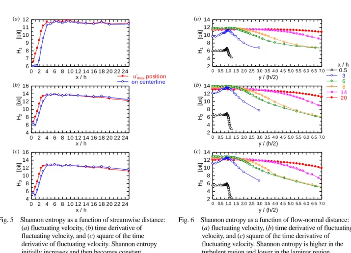
Fig. 5 Shannon entropy as a function of streamwise distance: (a) fluctuating velocity, (b) time derivative of fluctuating velocity, and (c) square of the time derivative of fluctuating velocity. Shannon entropy initially increases and then becomes constant.
Fig. 6 Shannon entropy as a function of flow-normal distance: (a) fluctuating velocity, (b) time derivative of fluctuating velocity, and (c) square of the time derivative of fluctuating velocity. Shannon entropy is higher in the turbulent region and lower in the laminar region. 0 2 4 6 8 10 12 14 16 18 20 22 24 4 6 8 10 12 14 16 x / h H2 [ b it ] (b) 0 2 4 6 8 10 12 14 16 18 20 22 24 4 6 8 10 12 14 16 x / h H3 [ b it ] (c) 0 2 4 6 8 10 12 14 16 18 20 22 24 6 7 8 9 10 11 12 x / h H1 [ b it ] u'max position on centerline (a) 0 0.5 1.0 1.5 2.0 2.5 3.0 3.5 4.0 4.5 5.0 5.5 6.0 6.5 7.0 2 4 6 8 10 12 14 y / (h/2) H2 [ b it ] (b) 0 0.5 1.0 1.5 2.0 2.5 3.0 3.5 4.0 4.5 5.0 5.5 6.0 6.5 7.0 2 4 6 8 10 12 14 y / (h/2) H1 [ b it ] x / h 0.5 3 6 8 14 20 (a) 0 0.5 1.0 1.5 2.0 2.5 3.0 3.5 4.0 4.5 5.0 5.5 6.0 6.5 7.0 2 4 6 8 10 12 14 y / (h/2) H3 [ b it ] (c)
なお,局所の中心速度などを用いて無次元化して考察することも重要なことであるが,次節以後で求めるシャ ノンエントロピー,順列エントロピーや,近似コルモゴロフ複雑度は,いずれも局所の諸量の最大値と最小値間 での分布様式を解析するものであるから,原物理量の無次元化方法の影響は受けない. 4・2 シャノンエントロピー 図4 にシャノンエントロピーの x-y 平面上のコンターを示す.また図 5 に中心線 y/(h/2) = 0 上(青○印),及び 各 x における変動速度rms 値 u’の y 方向分布において最大となる位置(赤●印)におけるシャノンエントロピー の x 方向変化を示す.図6 には代表的な 6 つの x におけるシャノンエントロピーの y 方向変化を示す. シャノンエントロピーの値は層流では小さく乱流では大きいが,H1,H2,H3いずれも分布様式は大きくは変わ らない.すなわち確率分布は u と∂u/∂t では大きくは変わらないことを示唆している.しかし図5 から,下流方向 への変化を調べると,H1(図5(a))よりも H2(図5(b)),さらに H3(図5(c))になると減少がやや激しい. そこで中心線上でシャノンエントロピーが大きい x/h = 6, y / (h/2) = 0 と下流の x/h = 25, y / (h/2) = 0 の二つの位 置における確率分布を考察する.図7 に 3 量の確率分布を示す.横軸は例えば図 7(a)では u と記しているが,実 際はこれは熱線出力電圧であり,無次元化せずに表示しているので単位は[V]となる.各横軸位置における鉛直線 の高さが確率であり,各図中の全鉛直線高さの合計が1 である. まず∂u/∂t のグラフ(図7(b))と(∂u/∂t)2のグラフ(図7(c))の形状について考えてみる.今ある確率変数 X の確 率密度関数を fX(x)とする.もう一つの確率変数 Y が X の関数であるとし,それが Y = f(X)と与えられているとき, Y の密度関数 fY(y)の形を調べる問題は Papoulis の本(1965)に示されている.それが Y = aX 2 の場合には同書の式(5-9)であり,読者の便宜のためにここに引用する次式である.
𝑓
𝑌(𝑦) =
2√𝑎𝑦1[𝑓
𝑋(√
𝑦𝑎) + 𝑓
𝑋(−√
𝑦𝑎)] 𝑈(𝑦)
(10) ここに U(y)はヘビサイド関数である.本実験の場合,図 7(a), (b)に見られるように問題の分布はガウス分布の形 で,この Y = aX 2の分布は同書によれば次式で与えられる.𝑓
𝑌(𝑦) = [
𝜎√2𝜋𝑎𝑦1𝑒𝑥𝑝(
2𝑎𝜎−𝑦2)]𝑈(𝑦)
(11) 上式で分かるように,fY(y)は y > 0 でのみ存在し,y → 0 では 1/√𝑦 の形で無限大に発散し,y → ∞では 0 に漸 近する.これに対応した変化が明らかに図7(c)の形状に見られる. -4 -3 -2 -1 0 1 2 3 4 0 0.0002 0.0004 0.0006 0.0008 0.0010 u [V] p1 (a) -4 -3 -2 -1 0 1 2 3 4 0 0.0001 0.0002 0.0003 0.0004 0.0005 ∂u/∂t [V/s] p2 (b) ×103 0 1 2 3 4 5 6 7 8 9 10 0 0.0005 0.0010 0.0015 0.0020 (∂u/∂t)2 [V 2/s2] p3 (c) ×106Fig. 7 Probability distribution: (a) fluctuating velocity, (b) time derivative of fluctuating velocity, and (c) square of the time derivative of fluctuating velocity. Green, x/h = 6, y/(h/2) = 0; red, x/h = 25, y/(h/2) = 0. Distribution widths become narrower downstream.
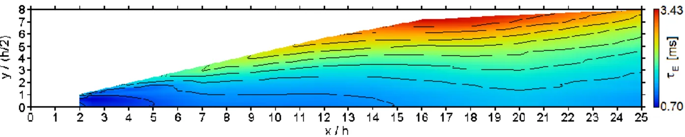
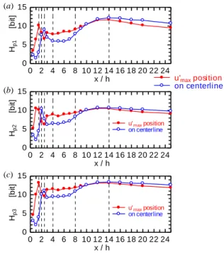
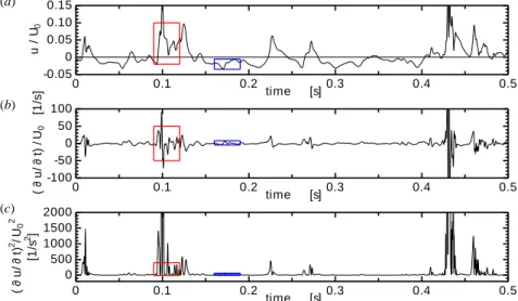
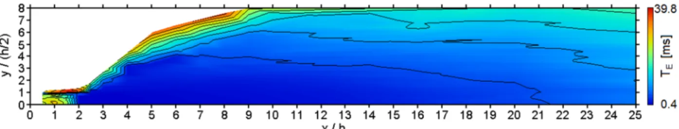
次に図 7 において下流方向への変化(緑色分布から赤色分布への変化)を見る.図 3(a)に現れているように u’ すなわち u の変動幅が減少するために確率分布の幅(横軸上の分布範囲)が減る.このため,式(1)における確率 事象数 n が減少するためにシャノンエントロピーは減少する.そして確率分布幅の減少は,u 自身よりもその時 間変化∂u/∂t(図 7(b))や(∂u/∂t)2(図 7(c))の方が激しい.これは時間スケールの代表として図 8 に示す Taylor の 微小時間スケールE が特に等値線からわかるように,混合層周辺付近になると(x/h 一定では y / (h/2)が増加する と)大きく増加することに加え,下流でも(y / (h/2)一定では x/h が増加しても)やや増加することからわかるよ うに,下流では上流よりも変動の時間スケールが長くなることから裏付けられる.このことは前述のように図 3(b), (c)の変動渦度や乱れエネルギー散逸率が x/h≒20, y/(h/2)≒0 において減少していることにも反映する.図 8 は, Taylor の微小時間スケールの分布を示したものである.ただしこれが大きいポテンシャルコア内の層流や混合層 外端を除き,2≦x/h 及び 0.1≦U / Umの範囲において描いた.なお後の図 17 に示す変動速度の積分時間も下流に 行くと増加する. 4・3 順列エントロピー 正規化しない順列エントロピーのコンターを図 9 に示す.また,図 10 に中心線上(青○印),及び各 x におけ る変動速度 rms 値 u’の y 方向分布において最大となる位置(赤●印)における x 方向変化を示し,図 11 に代表的 な 6 つの x における y 方向変化を示す.シャノンエントロピーと同様に,u,∂u/∂t,(∂u/∂t)2の順列エントロピーH p にそれぞれ 1,2,3 の下付添字を付す.なお前報(一宮,中村,2017)では n – 1 で正規化した u の順列エントロピ ーを掲載したが,これは本図 9~11 の Hp1の値を 7 で除したものに相当する. u の順列エントロピーHp1(図 9(a))は下流方向に単調に変化しないが,これは変動速度などの時系列変化のパ ターンが下流方向に複雑に変化するためである.その過程は前報(一宮,中村,2017)で詳述した.さて,Hp1はポ テンシャルコアが存続している x/h≦5 では混合層中心(y/(h/2) = 0)付近では小さく,ノズル端面(y/(h/2) = 1) 付近では大きいが,ポテンシャルコアが消滅してからは混合層中心で大きい.しかし∂u/∂t や(∂u/∂t)2の順列エント ロピーHp2,Hp3(図 9(b),(c))は混合層中心ではなく周辺部(6≦x/h≦18 の 4≦y / (h/2)≦8)において大きい. これはその x/h における変動速度 rms 値 u’が最大となる y / (h/2)の 3~4 倍の位置となる.この理由を以下で考察 する. Hp2,Hp3が小さい混合層中心部の代表として x/h = 5, y/(h/2) = 0 を,大きい周辺部の代表として x/h = 12, y/(h/2) = 6.6 を選ぶ.図 12, 13 に両位置における u, ∂u/∂t, (∂u/∂t)2 の瞬時波形を描く.中心部(図 12)では 3 量ともに常に 変動しており,しかも基本周波数や高調波周波数,低調波周波数が認められる周期的な変動である.そのため隣 り合うデータの値の大小関係のパターン(順列パターン)は少なくなって,これが順列エントロピーが小さくな ることに寄与する.これに対して周辺部(図 13)では間欠的に乱れた u 波形(a)が見られ,これに伴い∂u/∂t (b)と (∂u/∂t)2 (c)も間欠的に大きくなる.そのため順列パターンは多くなり,順列エントロピーは大きくなる.このこと は変動 u 自身よりも,それを時間微分した∂u/∂t や(∂u/∂t)2の方に敏感に表れる. しかし,同じく間欠的な波形であるのに,周辺部ではなぜ Hp1は小さく,Hp2や Hp3は大きいかを,さらに詳し く調べる.図 13 波形中から,激しく変動する区間[0.09 s, 0.12 s]と変動がおだやかな区間[0.16 s, 0.19 s]の,いずれ も 0.03 秒間を選び出した.これは図 13 中にそれぞれ赤色と青色の長方形枠で囲んでいる部分である.その長方 形枠部を拡大した図を,それぞれ図 14 と図 15 に示す.ここでは A/D 変換のサンプルデータ点も〇印で示す.
Fig. 8 Contour map of Taylor micro timescale in the x–y plane. Nine contour lines are drawn with 10 equal intervals between the maximum and minimum values. Except for the peripheral region with small turbulence, the timescale increases downstream.
Fig. 9 Contour map of dimensional permutation entropy in the x–y plane, n = 8: (a) fluctuating velocity, (b) time derivative of fluctuating velocity, and (c) square of the time derivative of fluctuating velocity. Nine contour lines are drawn with 10 equal intervals between the maximum and minimum values. The permutation entropy in the peripheral region of the mixing layer is high.
Fig. 10 Dimensional permutation entropy as a function of
streamwise distance, n = 8: (a) fluctuating velocity, (b) time derivative of fluctuating velocity, and (c) square of the time derivative of fluctuating velocity. The permutation entropy initially increases and then decreases and subsequently increases again in the streamwise direction. It finally decreases downstream.
Fig. 11 Dimensional permutation entropy as a function of
flow-normal distance, n = 8: (a) fluctuating velocity, (b) time derivative of fluctuating velocity, and (c) square of the time derivative of fluctuating velocity. The permutation entropy is higher in the turbulent region and lower in the laminar region.
0 2 4 6 8 10 12 14 16 18 20 22 24 0 5 10 15 x / h Hp3 [ b it ] u'max position on centerline (c) 0 2 4 6 8 10 12 14 16 18 20 22 24 0 5 10 15 x / h Hp1 [ b it ] u'max position on centerline (a) 0 2 4 6 8 10 12 14 16 18 20 22 24 0 5 10 15 x / h Hp2 [ b it ] u'max position on centerline (b) 0 0.5 1.0 1.5 2.0 2.5 3.0 3.5 4.0 4.5 5.0 5.5 6.0 6.5 7.0 0 5 10 15 y / (h/2) Hp3 [ b it ] (c) 0 0.5 1.0 1.5 2.0 2.5 3.0 3.5 4.0 4.5 5.0 5.5 6.0 6.5 7.0 0 5 10 15 y / (h/2) Hp1 [ b it ] x / h 0.5 3 6 8 14 20 (a) 0 0.5 1.0 1.5 2.0 2.5 3.0 3.5 4.0 4.5 5.0 5.5 6.0 6.5 7.0 0 5 10 15 y / (h/2) Hp2 [ b it ] (b)
0 0.1 0.2 0.3 0.4 0.5 -0.5 0 u / U time [s] 0 0.1 0.2 0.3 0.4 0.5 -1000 -500 0 500 1000 (∂ u/ ∂ t) /U 0 [ 1 /s] (b) time [s] 0 0.1 0.2 0.3 0.4 0.5 0 1 2 3 4 (∂ u/ ∂ t) 2 / U0 2 (c) time [s] ×105 [1 /s 2 ]
Fig. 12 Fluctuating signals, x/h = 5, y/(h/2) = 0: (a) fluctuating velocity, (b) time derivative of fluctuating velocity, and (c) square of the time derivative of fluctuating velocity. The signals always fluctuate leading to an increase in the permutation patterns. 0 0.1 0.2 0.3 0.4 0.5 -0.05 0 0.05 0.10 0.15 u / U 0 (a) time [s] 0 0.1 0.2 0.3 0.4 0.5 -100 -50 0 50 100 (∂ u/ ∂ t) / U0 [ 1 /s] (b) time [s] 0 0.1 0.2 0.3 0.4 0.5 0 500 1000 1500 2000 (∂ u/ ∂ t) 2/ U0 2 (c) time [s] [1 /s 2 ]
Fig. 13 Fluctuating signals, x/h = 12, y/(h/2) = 6.6: (a) fluctuating velocity, (b) time derivative of fluctuating velocity, and (c) square of the time derivative of fluctuating velocity. The signals fluctuate intermittently leading to an increase in the permutation patterns. 0.090 0.095 0.100 0.105 0.110 0.115 0.120 -0.020 0.02 0.04 0.06 0.08 0.10 u / U 0 (a) time [s] 0.090 0.095 0.100 0.105 0.110 0.115 0.120 -40 -20 0 20 40 (∂ u/ ∂ t) / U0 [ 1 /s] (b) time [s] 0.090 0.095 0.100 0.105 0.110 0.115 0.120 0 100 200 300 400 (∂ u/ ∂ t) 2 / U0 2 (c) time [s] [1 /s 2 ]
Fig. 14 Fluctuating signals with violent fluctuation, x/h = 12, y/(h/2) = 6.6: (a) fluctuating velocity, (b) time derivative of fluctuating velocity, and (c) square of the time derivative of fluctuating velocity. The signals fluctuate intermittently leading to an increase in the permutation patterns.
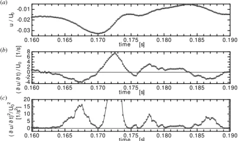
変動が激しい区間(図14)では,取り出すデータ数 n = 8 個中では,u 波形(a)は単調に変化することが多い. これに対して∂u/∂t 波形(b)は単調変化が少なくなり,さらに(∂u/∂t)2波形(c) は単調変化がかなり減るので順列パタ ーンは多くなり,このため順列エントロピーは大きくなることが裏付けられる. 一方,変動がおだやかな区間(図15)においても,u 波形(a)は n = 8 個中には単調に変化することが多いこと がわかる.これに対して∂u/∂t 波形(b)は細かい増減が見られ,単調に変化していないことがわかる.さらに(∂u/∂t)2 波形(c) も単調に変化しないことがわかる.この x/h = 12, y/(h/2) = 6.6 において,T – n +1((a)は 262144 – 8 + 1 = 262137 個,(b),(c)は 262140 – 8 + 1 = 262133 個)中から取り出した 8 個のデータの順列が,単調に減少する確率と 単調に増加する確率の和は,u では18.7%だが,∂u/∂t では7.5%,また(∂u/∂t)2では4.3%と少ない.以上のように間 欠的な乱流領域では,変動速度自体よりもその時間微分やさらにその2 乗の方が,データ間のすなわち時間に対 する変化様式が複雑になる.これが図9~11 の順列エントロピー分布に現れる.このような現象の流体力学的な 説明は今後の課題である. なお変動速度の間欠性は,扁平度 F = 𝑢4̅ (𝑢/ 2̅ )2 に反映する.そこで図 16 に u の扁平度のコンターを示す.扁 平度が大きい領域は,Hp2や Hp3が大きい領域とほぼ一致する. 4・4 順列エントロピー計算条件の検討 4・3 節で前述した順列エントロピーがシャノンエントロピーとは異なって,下流方向に単調に変化しない理由 をここで要約すると,最初の増加は変動速度の増加のためである.次の減少は,変動速度のさらなる増加のため に,取り出しデータ数 n = 8 の数列内では単調増加または単調減少が優勢になって変化パターン(順列パターン)
Fig. 16 Contour map of flatness factor of the streamwise fluctuating velocity in the x–y plane. Nine contour lines are drawn with 10 equal intervals between the maximum and minimum values. The flatness factor is high in the peripheral region of the mixing layer.
Fig. 15 Fluctuating signals with moderate fluctuation, x/h = 12, y/(h/2) = 6.6: (a) fluctuating velocity, (b) time derivative of fluctuating velocity, and (c) square of the time derivative of fluctuating velocity. The signals fluctuate intermittently leading to an increase in the permutation patterns.
0.160 0.165 0.170 0.175 0.180 0.185 0.190 -0.03 -0.02 -0.01 u / U0 (a) time [s] 0.160 0.165 0.170 0.175 0.180 0.185 0.190 -4 -20 2 4 6 8 (∂ u /∂ t) / U0 [ 1 /s ] (b) time [s] 0.160 0.165 0.170 0.175 0.180 0.185 0.190 0 5 10 15 20 (∂ u /∂ t) 2 / U0 2 (c) time [s] [1 /s 2 ]
がかえって減少するためである.最後の増加は変動速度において不規則変動が支配的になって順列パターンが増 えるためである. このように順列エントロピーが単調に変化しない原因は,全データとも n を一定値8 に保ったためである可能 性があるので,本節ではこれを局所の流れの時間スケールに応じて変化させることを検討した. 用いる時間スケールとしては,Taylor の微小時間スケールτE(図8)と積分時間(図 17) TE =
∫
𝑢(𝑡)𝑢(𝑡+𝜏)̅̅̅̅̅ 𝑢2̅ ∞ 0 dτ
(12) を検討した.両時間の分布様式は大まかには似ており,混合層の周辺部(y/(h/2)大)では両時間ともに増加する. しかし x/h = 20 よりも下流に行くと分布様式は異なり,20≦x/h≦25 において Taylor 微小時間はやや減少するが 積分時間は最後まで増加する.このような下流への大渦時間スケールの増加を考慮して,データ取り出し時間に は積分時間を採用した.具体的には,積分時間をサンプリング時間間隔で除して四捨五入した整数を区間数に等 しく設定した.ゆえに,これに1 を加えたものが取り出しデータ数 n になる.これはとても大きな値になるので, 計算機能力の制約のために n = 86(TE≒17 ms)を最大として計算した.図 17 からわかるように TEが17 ms より も大きくなるのは周辺部のみであるし,前報(一宮,中村,2017)に示したように n がある程度大きくなると順列 エントロピーは飽和するので,問題ないと思われる. 以上のように計算した順列エントロピーのコンターを図18 に示す.また,図 19 に中心線上(青○印),及び各 x における変動速度rms 値 u’の y 方向分布において最大となる位置(赤●印)における x 方向変化を示し,図 20 に代表的な6 つの x における y 方向変化を示す.なお n – 1 で正規化すると,前報(一宮,中村,2017)に示したよ うに n がある程度大きくなると順列エントロピーが飽和するにもかかわらず,大きな n – 1 で除した値が得られ るので,分布形状は奇妙なものになる.そこで正規化しない分布のみを本論文では載せる. 分布は全体的に,下流への乱流遷移の進行に伴って単調に増加する.n = 8 に固定した順列エントロピー(図 9 ~11)では存在した,Hp2や Hp3の周辺部での極大はここでは見られない.これは前述したように n が大きいと順 列エントロピーが飽和するため,周辺部も中心部も積分時間が大きいことに伴って順列エントロピーが十分大き いほぼ等しい値となったのである.このように周辺部の間欠的な信号は取り出し個数を変化させた順列エントロ ピーには反映しなくなる.またノズル出口直後の x/h = 0.5 での値からいったん減少して 2.5≦x/h≦5 で最少と なった後に,ポテンシャルコア消滅後は乱流遷移の進行に応じて増加する.このように,乱流遷移の進行ととも にいったん減少した後に増加するという特性は,佐藤の雑然度(Sato and Saito, 1975)と同じであり,単調に変化す る遷移進行の測度を見出すという目的は満足されない.4・5 コルモゴロフ複雑度
図21 に,u,∂u/∂t,(∂u/∂t)2の近似コルモゴロフ複雑度AK のコンターを示す.また,図 22 に中心線上(青○
印),及び各 x における変動速度rms 値 u’の y 方向分布において最大となる位置(赤●印)における x 方向変化を 示し,図23 に代表的な 6 つの x における y 方向変化を示す.
Fig. 17 Contour map of integral time of the streamwise fluctuating velocity in the x–y plane. Nine contour lines are drawn with 10 equal intervals between the maximum and minimum values. The integral time increases downstream.
Fig. 18 Contour map of dimensional permutation entropy in the x–y plane, n varies according to the integral time: (a) fluctuating velocity, (b) time derivative of fluctuating velocity, and (c) square of the time derivative of fluctuating velocity. Nine contour lines are drawn with 10 equal intervals between the maximum and minimum values. The permutation entropy in the peripheral region of the mixing layer is high.
Fig. 20 Dimensional permutation entropy as a function of flow-normal distance, n varies according to the integral time: (a) fluctuating velocity, (b) time derivative of fluctuating velocity, and (c) square of the time derivative of fluctuating velocity. The permutation entropy is higher in the turbulent region and lower in the laminar region.
0 2 4 6 8 10 12 14 16 18 20 22 24 0 4 8 12 16 20 x / h Hp3 [ b it ] (c) 0 2 4 6 8 10 12 14 16 18 20 22 24 0 4 8 12 16 20 x / h Hp1 [ b it ] u'max position on centerline (a) 0 2 4 6 8 10 12 14 16 18 20 22 24 0 4 8 12 16 20 x / h Hp2 [ b it ] (b) 0 0.5 1.0 1.5 2.0 2.5 3.0 3.5 4.0 4.5 5.0 5.5 6.0 6.5 7.0 0 4 8 12 16 20 y / (h/2) Hp3 [ b it ] (c) 0 0.5 1.0 1.5 2.0 2.5 3.0 3.5 4.0 4.5 5.0 5.5 6.0 6.5 7.0 0 4 8 12 16 20 y / (h/2) Hp1 [ b it ] (a) x / h 0.5 3 6 8 14 20 0 0.5 1.0 1.5 2.0 2.5 3.0 3.5 4.0 4.5 5.0 5.5 6.0 6.5 7.0 0 4 8 12 16 20 y / (h/2) Hp2 [ b it ] (b)
Fig. 19 Dimensional permutation entropy as a function of streamwise distance, n varies according to the integral time: (a) fluctuating velocity, (b) time derivative of fluctuating velocity, and (c) square of the time derivative of fluctuating velocity. The permutation entropy initially increases rapidly, then increases slowly, and eventually decreases in the streamwise direction.
Fig. 21 Contour map of approximated Kolmogorov complexity in the x–y plane: (a) fluctuating velocity, (b) time derivative of fluctuating velocity, and (c) square of the time derivative of fluctuating velocity. Nine contour lines are drawn with 10 equal intervals between the maximum and minimum values. The approximated Kolmogorov complexity in the turbulent region of the mixing layer is high.
Fig. 22 Approximated Kolmogorov complexity as a function of streamwise distance: (a) fluctuating velocity, (b) time derivative of fluctuating velocity, and (c) square of the time derivative of fluctuating velocity. The approximated Kolmogorov complexity initially increases rapidly, then increases slowly, and eventually decreases in the streamwise direction.
Fig. 23 Approximated Kolmogorov complexity as a function of flow-normal distance: (a) fluctuating velocity, (b) time derivative of fluctuating velocity, and (c) square of the time derivative of fluctuating velocity. The approximated Kolmogorov complexity is higher in the turbulent region and lower in the laminar region. 0 2 4 6 8 10 12 14 16 18 20 22 24 0 0.1 0.2 0.3 0.4 0.5 x / h AK 3 (c) 0 2 4 6 8 10 12 14 16 18 20 22 24 0 0.1 0.2 0.3 0.4 0.5 x / h AK 1 u'max position on centerline (a) 0 2 4 6 8 10 12 14 16 18 20 22 24 0 0.1 0.2 0.3 0.4 0.5 x / h AK 2 (b) 0 0.5 1.0 1.5 2.0 2.5 3.0 3.5 4.0 4.5 5.0 5.5 6.0 6.5 7.0 0 0.1 0.2 0.3 0.4 0.5 y / (h/2) AK 2 x / h 0.5 3 6 (b) 8 14 20 0 0.5 1.0 1.5 2.0 2.5 3.0 3.5 4.0 4.5 5.0 5.5 6.0 6.5 7.0 0 0.1 0.2 0.3 0.4 0.5 y / (h/2) AK 1 (a) x / h 0.5 3 6 8 14 20 0 0.5 1.0 1.5 2.0 2.5 3.0 3.5 4.0 4.5 5.0 5.5 6.0 6.5 7.0 0 0.1 0.2 0.3 0.4 0.5 y / (h/2) AK 3 (c)
u の AK(本論文の記号 AK1)は既報(一宮,中村,2012)(Ichimiya and Nakamura, 2013)にも掲載した. AK3はポ テンシャルコア消滅後の値の増加は遅れ,乱流発達後の減少は早まる.これはシャノンエントロピーの変化と同 様に,下流での時間スケールの増大により変動が単純になるためである.すなわち細かい乱れは早く減衰して消 え,大きな構造が永く続くことをこれは示している. 以上のように,本研究では変動速度,その時間微分係数及びその 2 乗について,シャノンエントロピー,2 つ のデータ取り出し方法による順列エントロピー及び近似コルモゴロフ複雑度の変化を考察した.自由せん断流の 乱流遷移過程において単調に変化する測度を見出すという目的を完全に満足するものはなく,遷移過程自体も単 調に変化するわけではないこともあいまって,いまだ探究の余地がある. 5. 結 論 2 次元噴流出口に形成される混合層の層流-乱流遷移過程について,既報の変動速度に続いて,変動速度の時 間微分係数及びその 2 乗について,情報論的量を用いた解析及び複雑度解析を行い,以下の結論を得た. (1)シャノンエントロピーは,変動速度,変動速度の時間微分係数及びその 2 乗ともに分布様式に大差はないが, 下流での時間スケールの増加に対応して,変動速度の時間微分係数及びその 2 乗はやや減少する. (2)データ列からの取り出し個数を固定した順列エントロピーは,変動速度の時間微分係数及びその 2 乗は,混 合層周辺部においては,間欠的な速度波形を反映して大きくなる. (3)データ列からの取り出し個数を積分時間に応じて変化させた順列エントロピーは,ポテンシャルコア内では いったん減少し,ポテンシャルコア消滅後は乱流遷移の進行に対応して増加するが,混合層周辺部の間欠性は反 映しない. (4)近似コルモゴロフ複雑度の分布様式は変動速度のものよりも,その時間微分係数やさらにその 2 乗の方が値 は小さい.下流でも変動が単純になることによって,ポテンシャルコア消滅後の値の増加は遅れ,乱流発達後の 減少は早まる. 本実験の確率変数の 2 乗の分布に関する,名古屋大学酒井康彦教授の Papoulis の本のご教示に感謝する. 文 献
Bandt, C. and Pompe, B., Permutation entropy: A natural complexity measure for time series, Physical Review Letters, Vol. 88, No. 17 (2002), 174102.
Burattini, P., The effect of the X-wire probe resolution in measurements of isotropic turbulence, Measurement Science and Technology, Vol. 19, No. 11 (2008), 115405.
da Silva, C. B., Hunt, J. C. R., Eames, I. and Westerweel, J., Interfacial layers between regions of different turbulence intensity, Annual Review of Fluid Mechanics, Vol. 46 (2014), pp. 567–590.
del Álamo, J. C. and Jiménez, J., Estimation of turbulent convective velocities and correlations to Taylor’s approximation, Journal of Fluid Mechanics, Vol. 640 (2009), pp. 5–26.
Eames, I. and Flor, J. B., New developments in understanding interfacial processes in turbulent flows, Philosophical Transactions of the Royal Society, A, Vol. 369 (2011), pp. 702–705.
Geng, C., He, G., Wang, Y., Xu, C., Lozano-Durán, A. and Wallace, J. M., Taylor’s hypothesis in turbulent channel flow considered using a transport equation analysis, Physics of Fluids, Vol.27, Issue 2 (2015), 025111.
He, X., He, G. and Tong, P., Small-scale turbulent fluctuations beyond Taylor’s frozen-flow hypothesis, Physical Review E, Vol. 81, Issue 6 (2010), 0650303.
Higgins, C. W., Froidevaux, M., Simeonov, V., Vercauteren, N., Barry, C. and Parlange, M. B., The effect of scale on the applicability of Taylor’s frozen turbulence hypothesis in the atmospheric boundary layer, Boundary-Layer Meteorology, Vol.143, Issue 2 (2012), pp. 379–391.
Hinze, J. O., Turbulence, 2nd Edition (1975), p. 46, McGraw-Hill.
Hunt, J. C. R., Eames, I., da Silva, C. B. and Westerweel, J., Interfaces and inhomogeneous turbulence, Philosophical Transactions of the Royal Society, A, Vol. 369 (2011), pp. 811–832.
一宮昌司, 加藤敏宏, 森本努, 2次元噴流出口混合層に及ぼす局所周期撹乱の効果, 日本機械学会論文集 B 編, Vol. 77, No. 775 (2011a), pp. 424–436.
Ichimiya, M., Kato, T. and Morimoto, T., Effect of local periodic disturbance on mixing layer at exit of two-dimensional jet, Journal of Fluid Science and Technology, Vol. 6, No. 6 (2011), pp. 887–901.
一宮昌司, 中村育雄, コルモゴロフ複雑度による乱流のランダムさ表現(混合層の場合), 日本機械学会論文集 B 編, Vol. 78, No. 788 (2012), pp. 794–810.
Ichimiya, M., Kamada, S., Okajima, A. and Osaki, T., Effect of local periodic disturbance on mixing layer downstream of two-dimensional jet (Spatial structure and quantitative representation of laminar-turbulent transition process), Journal of Fluid Science and Technology, Vol. 8, No. 1 (2013), pp. 90–105.
一宮昌司,三浦武紘,鎌田慎也, 2次元噴流出口混合層に及ぼす局所周期撹乱の効果(撹乱振幅と周波数の影響), 日本機械学会論文集 B 編, Vol. 79, No. 806 (2013), pp. 2093–2108.
Ichimiya, M. and Nakamura, I., Randomness representation in turbulent flows with Kolmogorov complexity (In mixing layer), Journal of Fluid Science and Technology, Vol. 8, No. 3 (2013), pp. 407–422.
一宮昌司, 中村育雄,原達彦, コルモゴロフ複雑度による乱流のランダムさ表現(平板上単一突起下流の乱流くさ びの場合), 日本機械学会論文集, Vol. 80, No. 813 (2014), DOI: 10.1299/transjsme.2014fe0117.
Ichimiya, M., Sakai, H. and Oohara, T., Properties of the laminar-turbulent transition in a mixing layer by the low-frequency disturbance (Effect of the anti-symmetrical disturbance), Journal of Fluid Science and Technology, Vol. 9, No. 3 (2014), DOI: 10.1299/jfst.2014jfst0038.
一宮昌司, 中村育雄,田村和大, コルモゴロフ複雑度による乱流のランダムさ表現(円管助走部境界層の乱流遷移 の場合), 日本機械学会論文集, Vol. 81, No. 828 (2015), DOI:10.1299/transjsme.15-00172.
一宮昌司, 中村育雄,各種情報量を用いた混合層の層流―乱流遷移過程の解析, 日本機械学会論文集, Vol. 83, No. 845 (2017), DOI:10.1299/transjsme.16-00497.
金子晃,偏微分方程式入門 (1998), p. 102, 東京大学出版会.
Kolmogorov, A. N., Three approaches to the quantitative definition of information, Problems of Information Transmission, Vol. 1, No. 1 (1965), pp. 1–7.
Kolmogorov, A. N., Combinatorial foundations of information theory and the calculus of probabilities, Russian Mathematical Surveys, Vol. 38, No. 4 (1983), pp. 29–40.
Moin, P., Revisiting Taylor’s hypothesis, Journal of Fluid Mechanics, Vol.640 (2009), pp. 1–4. 中村育雄,大坂英雄,工科系 流体力学 (1985), p. 213, 共立出版.
Panton, R. L., Incompressible Flow, 3rd ed. (2005a), p. 717, John Wiley & Sons. Panton, R. L., Incompressible Flow, 3rd ed. (2005b), p. 749, John Wiley & Sons.
Papoulis, A., Probability, Random Variables, and Stochastic Processes (1965), pp. 125, 129–130, McGraw-Hill.(日本語訳, 平岡寛二,篠崎寿夫,天野正章,村田忠夫 共訳,工学のための応用確率論,基礎編 (1970), pp. 122, 126, 東 海大学出版会.)
Pope, S. B., Turbulent Flows (2000), pp. 223–224, Cambridge University Press.
Rotta, J. C. (Ferri, A., Kuchemann, D. and Sterne, L. H. G. ed.), Turbulent boundary layers in incompressible flow, Progress in Aeronautical Sciences, Vol. 2 (1962), p. 8, Pergamon Press.
Sato, H. and Saito, H., Fine-structure of energy spectra of velocity fluctuations in the transition region of a two-dimensional wake, Journal of Fluid Mechanics, Vol. 67, Part 3 (1975), pp. 539–559.
Schlichting, H. and Gersten, K., Boundary-Layer Theory, 8th Revised and Enlarged ed. (2000a), p. 13, Springer. Schlichting, H. and Gersten, K., Boundary-Layer Theory, 8th Revised and Enlarged ed. (2000b), p. 421, Springer.
Shannon, C. E., A mathematical theory of communication, The Bell System Technical Journal, Vol. 27 (1948), pp. 379–423, 623–656.
Shannon, C. E. and Weaver, W., The Mathematical Theory of Communication (1949), p. 18, University of Illinois Press.(日 本語訳,植松友彦訳,通信の数学的理論 (2009), p. 88,筑摩書房.)
Shet, C. S., Cholemari, M. R. and Veeravalli, S., Eulerian spatial and temporal autocorrelations: assessment of Taylor’s hypothesis and a model, Journal of Turbulence, Vol.18, No.12 (2017), pp. 1105–1119.
Taylor, G. I., The spectrum of turbulence, Proceedings of the Royal Society of London, Series A, Vol. 164, Issue 919 (1938), pp. 476–490.
Tsinober, A., Vedula, I. P. and Yeung, P. K., Random Taylor hypothesis and the behavior of local and convective accelerations in isotropic turbulence, Physics of Fluids, Vol.13, Issue 7 (2001), DOI: 10.1063/1.1375143.
Yang, X. I. A. and Howland, M. F., Implication of Taylor’s hypothesis on measuring flow modulation, Journal of Fluid Mechanics, Vol.836 (2018), pp. 222–237.
References
Bandt, C. and Pompe, B., Permutation entropy: A natural complexity measure for time series, Physical Review Letters, Vol. 88, No. 17 (2002), 174102.
Burattini, P., The effect of the X-wire probe resolution in measurements of isotropic turbulence, Measurement Science and Technology, Vol. 19, No. 11 (2008), 115405.
da Silva, C. B., Hunt, J. C. R., Eames, I. and Westerweel, J., Interfacial layers between regions of different turbulence intensity, Annual Review of Fluid Mechanics, Vol. 46 (2014), pp. 567–590.
del Álamo, J. C. and Jiménez, J., Estimation of turbulent convective velocities and correlations to Taylor’s approximation, Journal of Fluid Mechanics, Vol.640 (2009), pp. 5–26.
Eames, I. and Flor, J. B., New developments in understanding interfacial processes in turbulent flows, Philosophical Transactions of the Royal Society, A, Vol. 369 (2011), pp. 702–705.
Geng, C., He, G., Wang, Y., Xu, C., Lozano-Durán, A. and Wallace, J. M., Taylor’s hypothesis in turbulent channel flow considered using a transport equation analysis, Physics of Fluids, Vol.27, Issue 2 (2015), 025111.
He, X., He, G. and Tong, P., Small-scale turbulent fluctuations beyond Taylor’s frozen-flow hypothesis, Physical Review E, Vol. 81, Issue 6 (2010), 0650303.
Higgins, C. W., Froidevaux, M., Simeonov, V., Vercauteren, N., Barry, C. and Parlange, M. B., The effect of scale on the applicability of Taylor’s frozen turbulence hypothesis in the atmospheric boundary layer, Boundary-Layer Meteorology, Vol.143, Issue 2 (2012), pp. 379–391.
Hinze, J. O., Turbulence, 2nd Edition (1975), p. 46, McGraw-Hill.
Hunt, J. C. R., Eames, I., da Silva, C. B. and Westerweel, J., Interfaces and inhomogeneous turbulence, Philosophical Transactions of the Royal Society, A, Vol. 369 (2011), pp. 811–832.
Ichimiya, M., Kato, T. and Morimoto, T., Effect of local periodic disturbance on mixing layer at exit of two-dimensional jet, Transactions of the Japan Society of Mechanical Engineers, Series B, Vol. 77, No. 775 (2011a), pp. 424–436 (in Japanese). Ichimiya, M., Kamada, S., Okajima, A. and Osaki, T., Effect of local periodic disturbance on mixing layer downstream of
two-dimensional jet (Spatial structure and quantitative representation of laminar-turbulent transition process), Transactions of the Japan Society of Mechanical Engineers, Series B, Vol. 77, No. 779 (2011b), pp. 1457–1471 (in Japanese). Ichimiya, M., Kato, T. and Morimoto, T., Effect of local periodic disturbance on mixing layer at exit of two-dimensional jet,
Journal of Fluid Science and Technology, Vol. 6, No. 6 (2011), pp. 887–901.
Ichimiya, M. and Nakamura, I., Randomness representation in turbulent flows with Kolmogorov complexity (In mixing layer), Transactions of the Japan Society of Mechanical Engineers, Series B, Vol. 78, No. 788 (2012), pp. 794–810 (in Japanese). Ichimiya, M., Kamada, S., Okajima, A. and Osaki, T., Effect of local periodic disturbance on mixing layer downstream of
two-dimensional jet (Spatial structure and quantitative representation of laminar-turbulent transition process), Journal of Fluid Science and Technology, Vol. 8, No. 1 (2013), pp. 90–105.
Ichimiya, M., Miura, T. and Kamada, S., Effect of local periodic disturbance on mixing layer downstream of two-dimensional jet (Effect of amplitude and frequency of the disturbance), Transactions of the Japan Society of Mechanical Engineers, Series B, Vol. 79, No. 806 (2013), pp. 2093–2108 (in Japanese).
Ichimiya, M. and Nakamura, I., Randomness representation in turbulent flows with Kolmogorov complexity (In mixing layer), Journal of Fluid Science and Technology, Vol. 8, No. 3 (2013), pp. 407–422.
Ichimiya, M., Nakamura, I. and Hara, T., Randomness representation in turbulent flows with Kolmogorov complexity (In turbulence wedge developed from a single roughness element on a flat plate), Transactions of the JSME (in Japanese), Vol. 80, No. 813 (2014), DOI: 10.1299/transjsme.2014fe0117.
Ichimiya, M., Sakai, H. and Oohara, T., Properties of the laminar-turbulent transition in a mixing layer by the low-frequency disturbance (Effect of the anti-symmetrical disturbance), Journal of Fluid Science and Technology, Vol. 9, No. 3 (2014), DOI: 10.1299/jfst.2014jfst0038.
Ichimiya, M., Nakamura, I. and Tamura, T., Randomness representation in turbulent flows with Kolmogorov complexity (In laminar-turbulent transition due to periodic injection in an inlet boundary layer in a circular pipe), Transactions of the JSME (in Japanese), Vol. 81, No. 828 (2015), DOI:10.1299/transjsme.15-00172.
Kaneko, A., Introduction to partial differential equation (1998), p.102, University of Tokyo Press (in Japanese).
Kolmogorov, A. N., Three approaches to the quantitative definition of information, Problems of Information Transmission, Vol. 1, No. 1 (1965), pp. 1–7.
Kolmogorov, A. N., Combinatorial foundations of information theory and the calculus of probabilities, Russian Mathematical Surveys, Vol. 38, No. 4 (1983), pp. 29–40.
Moin, P., Revisiting Taylor’s hypothesis, Journal of Fluid Mechanics, Vol.640 (2009), pp. 1–4. Nakamura, I. and Osaka, H., Koukakei ryutairikigaku (1985), p. 213, Kyoritsu Shuppan (in Japanese). Panton, R. L., Incompressible Flow, 3rd ed. (2005a), p. 717, John Wiley & Sons.
Panton, R. L., Incompressible Flow, 3rd ed. (2005b), p. 749, John Wiley & Sons.
Papoulis, A., Probability, Random Variables, and Stochastic Processes (1965), pp. 125, 129–130, McGraw-Hill. Pope, S. B., Turbulent Flows (2000), pp. 223–224, Cambridge University Press.
Rotta, J. C. (Ferri, A., Kuchemann, D. and Sterne, L. H. G. ed.), Turbulent boundary layers in incompressible flow, Progress in Aeronautical Sciences, Vol. 2 (1962), p. 8, Pergamon Press.
Sato, H. and Saito, H., Fine-structure of energy spectra of velocity fluctuations in the transition region of a two-dimensional wake, Journal of Fluid Mechanics, Vol. 67, Part 3 (1975), pp. 539–559.
Schlichting, H. and Gersten, K., Boundary-Layer Theory, 8th Revised and Enlarged ed. (2000a), p. 13, Springer. Schlichting, H. and Gersten, K., Boundary-Layer Theory, 8th Revised and Enlarged ed. (2000b), p. 421, Springer.
Shannon, C. E., A mathematical theory of communication, The Bell System Technical Journal, Vol. 27 (1948), pp. 379–423, 623–656.
Shannon, C. E. and Weaver, W., The Mathematical Theory of Communication (1949), p. 18, University of Illinois Press. Shet, C. S., Cholemari, M. R. and Veeravalli, S., Eulerian spatial and temporal autocorrelations: assessment of Taylor’s
hypothesis and a model, Journal of Turbulence, Vol.18, No.12 (2017), pp. 1105–1119.
Taylor, G. I., The spectrum of turbulence, Proceedings of the Royal Society of London, Series A, Vol. 164, Issue 919 (1938), pp. 476–490.
Tsinober, A., Vedula, I. P. and Yeung, P. K., Random Taylor hypothesis and the behavior of local and convective accelerations in isotropic turbulence, Physics of Fluids, Vol.13, Issue 7 (2001), DOI: 10.1063/1.1375143.
Yang, X. I. A. and Howland, M. F., Implication of Taylor’s hypothesis on measuring flow modulation, Journal of Fluid Mechanics, Vol.836 (2018), pp. 222–237.