Kyushu University Institutional Repository
バイアスフロー音響ライナーの実験的,数値的及び 理論的研究
ラムダニ, スフィアン
https://doi.org/10.15017/2534452
出版情報:Kyushu University, 2019, 博士(工学), 課程博士 バージョン:
権利関係:
Experimental, Numerical and Theoretical Study of Bias Flow Acoustic Liners
Supervisor: Prof. Nobuhiko Yamasaki
Examiners: Prof. Ken-ichi Abe
Prof. Masato Furukawa
Soufiane Ramdani
Kyushu University, Graduate School of Engineering Department of Aeronautics and Astronautics
2019/07
i
Acknowledgments
My deep thanks go to my supervisors in the Aerospace Propulsion Laboratory Prof.
Yamasaki and Mr. Inokuchi, for their guidance and recommendations and for their extraordinary support and patience all along the duration of this research.
I would like to express my gratitude to Dr. Ishii and Dr. Nagai from Japan Aerospace Exploration Agency for their numerous discussions and recommendations on different research matters.
I would like to thank Prof. Ken-ichi Abe and Prof Masato Furukawa for taking the time to examine this thesis.
I also wishes to thank Kyushu University faculty responsible for the education of the Aeronautics and Astronautics engineering students.
I would like to thank Ms. Tanaka for providing experimental data for different acoustic liners.
Thanks to the JAXA team developing the CFD tool used in this research.
I would like to thank the engineering student office and particularly Ms. Oiwa for her considerable help and support.
I sincerely thank my parents and siblings for their encouragement and moral support despite the long distance between us.
This project would have been impossible without the opportunity offered to me by the MEXT Scholarship program.
The computation was mainly carried out using the computer facilities at the Research Institute for Information Technology in Kyushu University.
ii
I. Introduction ... 1
1. Background ... 1
1.1. Engine Noise ... 1
Noise certification regulation ... 1
Noise sources ... 3
1.2. Combustion instabilities ... 4
1.3. Noise reduction technologies ... 6
2. Literature Survey ... 9
II. Numerical Methods ...12
1. Conservation Laws governing Fluid Dynamics ...13
2. Calculation method ...15
2.1. Finite volume method...15
2.2. Second order central difference ...18
2.3. Compact schemes ...20
2.4. Third order Runge-Kutta time integration ...25
3. Large Eddy simulation ...26
3.1. Spatial Filtering in LES ...26
3.2. Explicit and implicit sub-grid scale models ...27
3.3. Filtered Navier Stokes equations in upacs-LES ...29
4. Implementation of the sources ...32
4.1. Sound source ...32
4.2. Mass source ...34
III. Post-Processing Methods ...36
1. Transfer Function Method ...36
2. Viscous dissipation method ...41
3. Tecplot ...43
IV. Impedance tube Experiment ...44
1. Experimental configuration ...44
2. Perforated plates ...47
3. Conduction of the experiment ...50
iii
V. 2D Numerical Simulations ...56
1. Numerical Simulation of 2D acoustic liner based on our experiments ...56
1.1. Models and grid ...56
1.2. Numerical results and discussion ...60
1.2.1. Absorption coefficient. ...60
1.2.2. Flow field. ...62
2. Numerical Simulation of 2D acoustic liner based on Tam’s experiments ...68
2.1. Models and grid ...68
2.2. Numerical results and discussion ...71
2.2.1. Symmetry assumption verification ...71
2.2.2. Absorption coefficient ...76
2.2.2.1. Numerical Simulation of 2D Conventional Acoustic Liner ...76
2.2.2.2. Numerical Simulation of 2D Active Acoustic Liner with a Bias Flow ...77
2.2.3. Flow field ...79
2.2.3.1. Flow-field of the Conventional Acoustic Liner ...79
2.2.3.2. Flow-field of the Active Acoustic Liner with a Bias Flow ...81
VI. Theoretical study of acoustic liners ...82
1. Derivation of the wave equation and Webster’s horn equation ...82
1.1. Continuity equation...82
1.2. Momentum equation ...83
1.3. Webster horn equation ...84
1.4. Wave equation ...85
1.5. Helmholtz-like equation for Webster’s horn equation ...86
2. Helmholtz resonator ...86
3. Conventional slit resonator model ...87
4. Absorption of sound by a perforated screen with a backing cavity ...88
5. Modified models based on Hughes and Dowling model ...90
5.1. Straight aperture model ...90
5.2. Tapered aperture model ...91
5.3. Impedance model of the slit tapered aperture with bias flow ...94
iv
5.4.1. Straight aperture without bias flow ...95
5.4.2. Straight aperture with bias flow ...95
5.5. Theoretical model results for the slit tapered aperture ...98
5.5.1. Tapered aperture without bias flow ...98
5.5.2. Tapered aperture with bias flow ...98
5.5.3. Effect of tapering slope 𝒎 ... 101
VII. Conclusion ... 103
Bibliography ... 105
Appendix A: Compact schemes in upacs-LES ... 108
A1. The Burgers equation ... 108
A2. Compact interpolation for convective terms ... 110
A3. Compact difference for viscous terms ... 112
A4. Compact filter ... 114
Appendix B: Boundary conditions in the solver upacs-LES ... 118
B1. Notations ... 118
B2. Summary of the theory of characteristics ... 118
B3. Subsonic inflow B. C. (entry_subsonic_riemann, entry_subsonic) ... 120
B4. Subsonic outflow B. C. (exit_subsonic) ... 122
B5. Farfield B. C. (farfield_subsonic) ... 123
B6. Mass-flow specified B. C. ... 125
B7. Farfield B. C. as a mass-flow specified B. C. ... 126
Appendix C: Two Microphone Method Matlab code ... 128
v x Coordinate along the i-direction y Coordinate along the j-direction z Coordinate along the k-direction u Velocity along the i-direction v Velocity along the j-direction w Velocity along the k-direction
xi Indicial notation of coordinate components ui Indicial notation of velocity components
Physical propriety
Filtered physical propriety
Favre filter operation of physical propriety
Quantity based on filtered variables Cutoff width
G
Filtering kernel
SGS Error introduced by the discretization
M Error introduced by the difference by the SGS model
N Truncation errorMSGS SGS model
t Time
p Pressure
Densityui Velocity component in the i-direction
ij Viscous stress tensor
ij Turbulent stress tensor Sij Strain tensorE Total energy
qj Heat flux vector
vi Cs Constant of Smagorinsky
ij Velocity gradient tensorVc Vreman constant
B Flow function
𝑅 Reflection coefficient
𝐼 Sound intensity
α Absorption coefficient
Viscous dissipation function 𝐷(𝑥, 𝑦, 𝑧) Time-averaged dissipation rate 𝐸 Acoustic power through the aperture
𝐸 Acoustic power through the impedance acoustic tube 𝐸 Acoustic power converted to viscous dissipation
ℎ Thickness of the perforated plated 𝐷 Width of the straight aperture
𝑙 Depth of the cavity
𝑊 Width of the cavity
𝑑 Distance between slits
𝑏 Width at the base of trapezoidal shape of the tapered aperture 𝑎 Width at the top of trapezoidal shape of the tapered aperture 𝑍 Characteristic impedance of air
𝑍 Total impedance of a Helmholtz resonator 𝑍 Impedance of the cavity of a Helmholtz resonator 𝑍 Impedance of the aperture of a Helmholtz resonator 𝑍 . Impedance of the straight aperture
𝑍 . Impedance of the tapered aperture 𝑟 Resistance of the aperture
𝑋 Reactance of the aperture
𝑓 Resonant frequency
𝛿 End correction
𝑚 Tapering slope
vii
𝑄 Volume flow rate through the aperture
𝑀 Bias flow Mach number
viii
List of Tables
Table II-1 Coefficients of the compact Filter ...23
Table IV-1 dimensions of the straight slit aperture ...48
Table IV-2 dimensions of the tapered slit aperture ...49
Table V-1 Sound source conditions. ...70
Table V-2 Absorption coefficients for resonator without bias flow ...71
Table V-3 Absorption coefficients for resonator with bias flow ...71
Table V-4 Symmetry ...72
ix
List of Figures
Figure I-1 Noise certification reference points [1] ... 2
Figure I-2 ICAO noise standards [2] ... 2
Figure I-3 Turbo fan noise sources [3] ... 3
Figure I-4 Airplane noise components [4] ... 4
Figure I-5 burner assembly damaged by combustion instability [6] ... 5
Figure I-6 New burner assembly [6]... 5
Figure I-7 Schematic of thermo-acoustic coupling in a combustion duct. ... 5
Figure I-8 Location of acoustic liners [32] ... 6
Figure I-9 Layout of acoustic liners. ... 8
Figure I-10 Acoustic liner with bias flow ... 8
Figure II-1 Coordinates at the center and surface boundaries ...17
Figure II-2 Example of grid and notation for inner points ...21
Figure II-3 Example of grid and notation for left boundary ...21
Figure II-4 Example of grid and notation for left boundary ...22
Figure II-5 Grid and notation for right boundary ...23
Figure II-6 Grid and notation for left boundary ...24
Figure III-1 Sound impedance tube with Transfer Function Method ...40
Figure III-2 Integration domain ...42
Figure IV-1 Acoustic impedance tube ...45
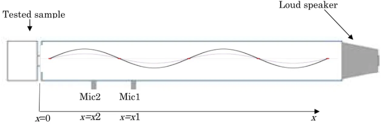
Figure IV-2 Schematic of the experimental setup ...45
Figure IV-3 Slit on the flange for outflow of jet ...46
Figure IV-4 Loud speaker ...46
Figure IV-5 Installation of microphones ...46
Figure IV-6 Model of active acoustic liner ...46
Figure IV-7 Straight aperture, unit: [mm] ...48
Figure IV-8 Tapered aperture, unit: [mm] ...49
Figure IV-9 Absorption coefficient for the straight aperture ...53
Figure IV-10 Absorption coefficient for the tapered aperture ...53
x
Figure IV-12 Resistance of the tapered aperture ...54
Figure IV-13 Reactance of the straight aperture ...55
Figure IV-14 Reactance of the tapered aperture ...55
Figure V-1 Layout of acoustic liners ...58
Figure V-2 Straight aperture...59
Figure V-3 Tapered aperture ...59
Figure V-4 Sources locations and boundary conditions ...59
Figure V-5 Absorption coefficients for the straight slit aperture ...61
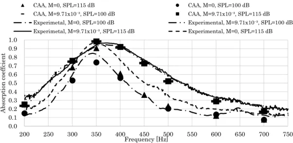
Figure V-6 Absorption coefficients for the tapered slit aperture ...61
Figure V-7 Non-dimensional vorticity magnitude, straight aperture, 350 Hz and 100 dB without bias flow ...64
Figure V-8 Non-dimensional vorticity magnitude, straight aperture, 350 Hz and 115 dB without bias flow ...64
Figure V-9 Non-dimensional vorticity magnitude, straight aperture, M=9.71× 𝟏𝟎 − 𝟑, 350 Hz and 100 dB ...64
Figure V-10 Non-dimensional vorticity magnitude, straight aperture, M=9.71× 𝟏𝟎 − 𝟑, 350 Hz and 115 dB ...64
Figure V-11 Non-dimensional vorticity, tapered aperture, 500 Hz and 100 dB without bias flow ...65
Figure V-12 Non-dimensional vorticity, tapered aperture, 500 Hz and 115 dB without bias flow ...65
Figure V-13 Non-dimensional vorticity magnitude, tapered aperture, M=9.71× 10 − 3, 500 Hz and 100 dB ...66
Figure V-14 Non-dimensional vorticity magnitude, tapered aperture, M=9.71× 10 − 3, 500 Hz and 115 dB ...66
Figure V-15 Time-averaged viscous dissipation, straight aperture, without bias flow 700 Hz, 115 dB t≅T/2 ...66
Figure V-16 Time-averaged viscous dissipation, tapered aperture, with-out bias flow 700 Hz, 115 dB, t≅T/2 ...67
Figure V-17 Boundary conditions of half resonator with symmetry assumption ...70
Figure V-18 Boundary conditions of full Resonator ...70
Figure V-19 Snapshots of the unsteady flow at the aperture: Vorticity contours-130 dB 1 kHz without bias flow ...72
Figure V-20 Snapshots of the unsteady flow at the aperture: Vorticity contours-150 dB 1 kHz without bias flow ...73
xi
Figure V-22 Snapshots of the unsteady flow at the aperture: Vorticity contours-150
dB 1 kHz with bias flow ...75
Figure V-23 Absorption coefficient: 130 dB ...78
Figure V-24 Absorption coefficient: 150 dB ...78
Figure V-25 Instantaneous non-dimensional viscous dissipation rate (VD): 150 dB, 1 kHz without bias flow ...80
Figure V-26 Percentage of the absorption caused by each term of the viscous dissipation term, cases without bias flow ...80
Figure VI-1 Mass flux ...82
Figure VI-2 Momentum flux ...83
Figure VI-3 Impedance decomposition of Helmholtz resonator ...87
Figure VI-4 Perforated plate with bias flow and backed by a cavity ...88
Figure VI-5 Perforated plate with straight aperture of finite thickness ...91
Figure VI-6 Perforated plate with tapered aperture ...91
Figure VI-7 Comparison of the absorption coefficient between experiment, CAA and theoretical models results: case without bias flow ...95
Figure VI-8 Comparison of the absorption coefficient between experiment, CAA and theoretical models results: with bias flow M=4.85× 10 − 3 ...96
Figure VI-9 Comparison of the absorption coefficient between experiment, CAA and theoretical models results: with bias flow M=9.71× 10 − 3 ...97
Figure VI-10 Comparison of the absorption coefficient between experiment, CAA and theoretical models results: with bias flow M=1.94× 10 − 2 ...97
Figure VI-11 Absorption coefficient for tapered slit aperture without bias flow ...98
Figure VI-12 Absorption coefficient for tapered slit aperture without bias flow M=4.85× 10 − 3 ...99
Figure VI-13 Absorption coefficient for tapered slit aperture with bias flow M=9.71× 10 − 3 ... 100
Figure VI-14 Absorption coefficient for tapered slit aperture with bias flow M=1.94× 10 − 2 ... 100
Figure VI-15 Absorption coefficient at different tapering slope ... 102
1
I. Introduction
During the last decades, the world had experienced a continuous increase in the development and manufacturing of airplanes due to the travel time reduction and the safety this means of transportation offers. Moreover, the introduction of low-cost carriers made it possible for a huge number of people to travel via airplanes, and thus increased the demand for airplanes. Air traffic has improved people’s quality of life and made it possible to shrink the world borders. Besides this, it also created thousands of jobs all around the world. However, this beneficial increase in air traffic was accompanied by an increase of multiple environmental pollutions.
One environmental pollution is the increase of greenhouse gases exhausted out of jet engines including a large amount of carbon dioxide which is detrimental to global warming, as well as pollutant emissions such as Nitrogen oxides NOx. Recent combustion chambers, aimed at low NOx emission and high combustion efficiency, tend to decrease the secondary air flow, which leads to increase the vibration in the combustion chambers caused by combustion instabilities.
The second environmental pollution is the noise produced by airplanes. Taking off and landing of large passenger airplanes are the noisiest periods during the flight which may influence on the comfort of people living in the residential areas around the airports.
The objective of this research is to study the acoustic liners used in turbofan engines to reduce the generated noise as well as the combustion instabilities, and to elucidate the influence of a bias flow passing through a perforated face sheet on the absorption capabilities of acoustic liners.
1. Background 1.1. Engine Noise
Noise certification regulation
The widespread usage of large passenger airplanes and the annoyance caused by their noise made it a necessity to quantify the noisiness of airplanes. The International Civil Aviation Organization (ICAO) is an agency of the United Nations, which ensures safe planning and development of international air transport, and the noise certification for airplanes is one of the missions that this agency deals with.
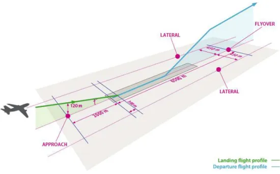
The Effective Perceived Noise level in decibel (EPNdB) is a number used to evaluate the loudness of an airplane for a human being on the ground, and it is calculated as the sum of the Effective Perceived Noise Level (a measure of sound level that takes into account the annoyance of spectral irregularities and the duration on human beings) on three different points situated nearby the runway as shown in Figure I-1:
- During takeoff at a microphone at a distance of 6.5km from the brake release.
- During takeoff at a microphone situated at a distance of 400m from the runway center - During landing at a microphone at a distance of 2km from the runway threshold.
2 Figure I-1 Noise certification reference points [1]
Figure I-2 shows the certification levels since the issuance of Chapter 2 (effective since 1972) until Chapter 14 (effective for all the new airplanes produced after 2017).
Chapter 4 is aiming to reduce the allowable SPL by 10dB over the limit of Chapter 3, and Chapter 14 is a revision of Chapter 4 in which the limit is reduced by 7dB compared to Chapter 4 and an extra elbow is added to the curve in order to account for the noise of lightweight airplanes, and this adds an extra constraint for lightweight airplane manufacturers.
Figure I-2 ICAO noise standards [2]
3
Such stricter standard has a role to motivate airplane and airplane engine manufacturers to continuously improve the existing noise reduction devices as well as to develop new technologies in order to meet the even stricter standard in the future.
Noise sources
For large passenger airplanes with turbofan engines, noise sources are classified into two, i.e., the primary noise source consist of the engines noise, while the secondary noise source is the airframe noise.
Figure I-3 shows the different sources of noise generated in the turbofan engines. The noise sources are classified into turbomachinery and jet sources.
The turbomachinery sources consist of the fan, compressor, combustor as well as turbine, whereas jet sources consist of the core mixing (mixing between hot-core and the fan-bypass air flows) and bypass mixing (mixing between the fan-bypass and surrounding air flows).
The fan noise consist of a broadband noise in addition to the tone noise. The tone noise is of high sound pressure level (SPL) and caused by the spinning of the fan with a specific frequency. Such that the fundamental frequency of the produced sound is the blade passing frequency BPF and it is calculated as the number of blades NR of the fan times its rotational speed .
BPFNR (I.1)
Figure I-3 Turbo fan noise sources [3]
4
Figure I-4 shows the levels of noise generated by different components of large passenger airplanes during takeoff and landing, and the main source of noise in the current airplanes is produced by the engines during takeoff. In addition to the engines, the airframe also produces a high noise level during landing due to the deployed flaps and landing gears in landing configurations.
Figure I-4 Airplane noise components [4]
Figure I-4 shows also that the highest noise is produced by the fan in case of approach while in the case of takeoff both jet and fan noises are predominant noise sources.
1.2. Combustion instabilities
In order to reduce exhausted pollutant emissions of Nitrogen oxides NOx out of jet engines, recent combustion chambers use lean premixed combustion technology.
The fuel and air are premixed in advance before entering the combustion chamber. This helps homogenize the mixture leading to more uniform temperature as well as a reduced flame temperature. Such a combustion results in low NOx emission and high combustion efficiency.
However, since the lean mixture is already rich in oxygen, contrary to old generation combustors, recent combustion chambers, aimed at low NOx emission and high combustion efficiency, tend to decrease the secondary air flow. This leads to undesirable combustion phenomena such as a lower stability flame and combustion dynamic phenomena giving rise to the vibration in combustion chambers, and one of these dynamic phenomena is the thermo- acoustic instabilities.
Figure I-5 shows a multi-burner assembly damaged by combustion instabilities as a result of lean premixed combustion. And Figure I-6 shows a new multi-burner assembly. These Figures show the irreversible damage that can occur to the combustor if combustor stability is not taken into account by dampening thermos-acoustic instabilities.
Figure I-7 show a schematic of a combustion duct were an unsteady flame results in generation of sound waves. Dynamic oscillations in the combustion chamber is related to conditions where a resonant coupling occurs between perturbations in the heat release and pressure field. In these conditions where the heat release perturbations is in phase with an acoustic wave, the results can be damaging as shown in Figure I-5. The aforementioned
5
condition is referred to as Rayleigh’s criterion. Putnam [5] formulated mathematically this criterion giving the following equation:
1
𝑇 𝑝 𝑞 𝑑𝑡 > 0 (I.2)
where 𝑝 denotes pressure fluctuations, 𝑞 denotes heat release oscillations and T is a period of time.
One of the methods to solve this thermo-acoustic instability problem is to dissipate the acoustic waves enough to eliminate the acoustic oscillations. This method is studied further in the present research.
Figure I-5 burner assembly damaged by
combustion instability [6] Figure I-6 New burner assembly [6]
Figure I-7 Schematic of thermo-acoustic coupling in a combustion duct.
6
1.3. Noise reduction technologies
Different means have been used in order to reduce the noise generated by turbofan engines such as installing chevrons or virtual chevrons [4] dealing with the jet noise, and acoustic liners in order to reduce fan noise [7]. In this study, we will focus on the conventional and active acoustic liners with bias flow.
Acoustic liners are used nowadays on most passenger airplanes because of their simplicity and effectiveness to attenuate fan noise.
Figure I-8 shows the locations where the acoustic liners are installed. For noise reduction, the main location is along the inner wall of the nacelle, and the liners installed in this area are conventional acoustic liners and have the main function of reducing the acoustic noise, however, the acoustic liners are also installed in the combustor in order to reduce combustion instabilities generated by acoustic waves. The liners in the combustor have a bias flow passing through the aperture, where bias flow is caused by the secondary air flow in the combustor.
Figure I-8 Location of acoustic liners [32]
7
As shown in Figure I-9, the acoustic liners consist of a perforated plate backed by a hard wall, with honeycomb support used to separate the two plates. They are fixed in the inner walls of the engine nacelle, in order to damp acoustic waves produced by the fan.
Conventional acoustic liners are known to well absorb acoustic energy in the range of frequency close to the resonance frequency. The noise produced by the engine, however, is broad, there comes the need for active acoustic liners, in order to optimally change the impedance of the liner to match the operating conditions of the engine. Various methods are used to technically realize active liners such as controllable piezoelectric [8] or bias flow [9]
which is the topic of the present study.
However active acoustic liners are still under investigation, an active method in this research refers to a method which adds mass, momentum or energy into the system, and these active methods are studied and developed to be further improved over the effectiveness of the conventional passive liner. Moreover, recent combustion chambers, aimed at low NOx emission and high combustion efficiency, tend to decrease the secondary air, which leads to increase the vibration in combustion chambers.
This is why understanding how to keep the attenuation or damping performance with little secondary air is important. To realize it, we study the attenuation mechanism of the bias flow type liners.
Figure I-10 shows an active acoustic liner where the blue arrows denote the direction of a bias flow passing through the backed plate.
The reason for which a steady bias flow is chosen can be made clear by considering the formulae of the rate of dissipation of acoustic energy given in the textbook by Howe [10].
∏ ≈ 𝜌 𝐮 ∙ (𝛚 × 𝐯)𝑑 𝐱 (I.3)
where 𝜌 is the density, 𝐮 is the acoustic particle velocity, 𝛚 is the vorticity, and 𝐯 is the velocity.
As demonstrated by Howe, the order of the term 𝛚 × 𝐯 is equal to 𝜀, the measure of the acoustic amplitude. Moreover the acoustic particle velocity 𝐮 only have the acoustic part and it is of the order of 𝜀, and as a result, the rate of production of vortical energy ∏ is of second order (~𝑂(𝜀 )). On the other hand, in the case of the acoustic model with no bias flow, both the velocity 𝐯 and the vorticity 𝛚 are of the order of 𝜀, thus 𝛚 × 𝐯 is of second order (~𝑂(𝜀 )), leading to the production of vortical energy ∏ of third order(~𝑂(𝜀 )). As a conclusion, the bias flow increases the rate of dissipation of acoustic energy in Eq. (I.3) by an order of magnitude.
8 Figure I-9 Layout of acoustic liners.
Cavity
Back wall
Perforated plate
Cavity
Back wall
Perforated plate
Bias flow
Figure I-10 Acoustic liner with bias flow
9
2. Literature Survey
Howe [11] theoretically proposed that a low frequency (low Strouhal number) sound wave can be significantly attenuated by a jet flow by converting the acoustical energy into energy of fluctuating vorticity, which is shed from the nozzle edge. Bechert [12] proposed another theory to explain this phenomenon, and this was supported via experimental data.
Bechert [12] also proposed a simple theory to predict the optimum Mach number of bias flow to obtain the perfect attenuation. On the other hand, Howe's theory to predict the sound absorption coefficient including the effects of a bias flow is well supported by an experiment by Hughes and Dowling [13]. Hence, this led to the idea that the off-resonant performance of a resonator can be improved if a jet (or a bias flow) is introduced from an aperture of an acoustic liner. Lahiri et al. [14] collected this type of experimental data and showed that the application of a bias flow through the aperture widens the frequency range of dissipation, with the penalty of reduced peak performance near the resonant frequency. Zhao and Li [15] wrote a summary on tunable acoustic liners including a liner with bias flow.
In the field of numerical simulation, Mendez et al. [16] performed a 3D simulation of a perforated plate with a circular aperture using the large eddy simulation (LES), and the results showed that LES can predict the acoustic behavior of resonators, and flow fields around the aperture can give an insight to the dissipation mechanism of acoustic liners.
Then Mendez applied a homogeneous model of multi-perforated plates to an actual gas turbine combustor chamber, where the walls contain huge amount of holes. This method represents a fast and practical alternative to include the influence of perforated plates to the simulation.
Ji and Zhao [17] performed a 2D lattice Boltzmann method (LBM) for an aperture with bias flow, and both made a comparison with Howe's theory, obtaining good agreements.
Roche et al. [18] conducted a 3D as well as 2D axisymmetric numerical simulation of cylindrical acoustic liner under a normal incidence acoustic wave for different frequencies as well as sound pressure levels. They used the Direct Numerical Simulation (DNS) and good agreement was obtained between the theoretical model, 2D and 3D models concerning the acoustic properties such as reflection and absorption coefficients for a low SPL of 80dB which is considered within the linear domain. However in the case of high sound pressure level of 150db where non-linearity has large influence, this linear theoretical model is not describing the acoustic behavior properly anymore, but good agreement is obtain between 2D and 3D models, and this shows that by opting for a 2D simulation, calculation time can be reduced enormously without a loss in the accuracy of the results. Also, it is observed that a wider absorption spectra and lower peaks are obtained.
DNS simulations were conducted by Tam et al. [19] for a 2D slit resonator of resonance frequency around 1 kHz for a range of frequencies of sound source from 1 kHz to 6 kHz and sound pressure levels of 130dB and 150dB. The absorption coefficients were obtained by evaluating the absorbed energy as the sum of the rate of viscous dissipation and the rate at which the energy is transferred to shed vortices. These simulations were validated by experiments using an acoustic impedance tube, in the same conditions. Good agreement
10
was obtained for the absorption coefficients, except for the case of sound source of 2 kHz and 130db where the experimental value is much larger than the simulation.
Tam et al. [19] distinguish two regimes with regard to the mechanisms through which the absorption phenomena occurs in acoustic liners:
- The low sound pressure level regime where the primarily mechanism of absorption is the viscous dissipation caused by the oscillatory boundary layer at the aperture of the perforated plate.
- The high-pressure level regime where vortices develop at the opening of the aperture then they are shed away. The absorption is caused by a conversion of acoustic energy to vortical energy that is dissipated later on by viscous effects.
Tam et al. [19] also conducted a series of experiments and Direct Numerical Simulation (DNS) to slit apertures with a 90° corner (straight aperture) and 45° corner (tapered aperture). The results obtained using the simulation supports the usage of computational aeroacoustics (CAA) as a design tool.
Zhang, Q et al. [20] studied a two-dimensional resonator under normal acoustic wave, using DNS, and he validated his results using experimental data by Tam, et al. [21], where he found that the results of the experiment and the simulation are in good agreement, also he worked on the problem including a grazing flow which models actual conditions in operating engines.
In the experimental field, Wada and Ishii [9] performed experiments for acoustic liners with a bias flow passing through the apertures of a perforated plate (circular straight perforations) and observed that the absorption range of the liner became wider and was not concentrated around the resonant frequency as in the case of the conventional liner.
They compared the experimental results with Howe's extended theory proposed by Luong et al. [22], which considered the thickness of the perforated sheet and obtained good agreements.
The macroscopic effect of the design parameters (such as the shape of the aperture and the flow velocity when a bias flow is applied through the aperture) on the impedance of an acoustic resonator was experimentally investigated via an acoustic impedance tube. The results revealed that the fully tapered aperture exhibited a wider absorption frequency range when compared to that of a straight circular aperture. However, little was known about the reason for such a behavior given the difficulty of visualizing the flow around the small apertures in the experimental setup using the impedance tube.
In the present study, the acoustic performance of the liner and the flow field around the perforated plate is numerically solved using the compressible Navier–Stokes equations to understand the acoustic and fluid dynamic behavior of the liner and the effect of the shape of the perforation at a microscopic level.
The aforementioned studies involve a long computational time and computational resources to perform 3D simulations. Thus, in the present study, the simulations are conducted using 2D large eddy simulations. For the 2D assumption to be acceptable, the impedance tube experiment is conducted on slit apertures where slit indicates that each plate has only one aperture with a high aspect ratio of 100. The aperture spans through the center of the plate. Subsequently, numerical simulations are conducted to focus on the
11
effect of bias flow on the absorption performance of the acoustic liner and flow field around the apertures.
In the next chapter, the details of the numerical code and the models used are explained, then the implementation of the sound source and mass source to generate the acoustic waves and the bias flow are given while in Chapter 3 the methods used for post- processing are explained.
In Chapter 4, the impedance tube experiment is conducted on slit apertures where slit indicates that each plate has only one aperture with a high aspect ratio of 100. The aperture spans through the center of the plate.
In Chapter 5, the numerical simulations conducted for conventional and active acoustic liners are validated with the results obtained from the experimental section. The simulations are conducted using 2D large eddy simulations, and are conducted to focus on the effect of bias flow on the absorption performance of the acoustic liner and flow field around the apertures.
In Chapter 6, the theoretical models are developed by modifying the model by Hughes and Dowling [23] for a screen with slit apertures in order to account for the thickness as well as the cross-section of the aperture of the plate. The results are then compared to the experimental and numerical results from the previous chapters.
Finally, few conclusions of the results obtained during this research are reported in Chapter 7.
12
Chapter 2
II. Numerical Methods
Nowadays numerical methods are widely used tools in many fields of engineering such as structural analysis, fluid dynamics, electromagnetic…, it is a mathematical field that implements algorithms in the interest of obtaining numerical solutions to problems defined by continuous functions.
The extensive use of these methods is for the reason that complex geometries that wouldn’t be solved analytically can be modeled numerically with usually a great accuracy for engineering purposes. In addition, the advent of supercomputers and the immense improvement of the calculation capabilities of computers made it possible to deal with much more complex problems along with a reduction in computational time.
This chapter intends to explain the numerical methods employed in this research. By understanding the physics and models in conjunction with the numerical schemes used, meaningful comparative conclusions can be drawn.
All the simulations in this study are carried out with the large eddy simulation (LES) code upacs-LES developed by Japan Aerospace Exploration Agency (JAXA), which solves the compressible Navier Stokes equations by Finite Volume Method for multi-block structured mesh.
The 6th-order compact scheme with the 10th-order compact filter is used to solve the convective terms of the conservation equations, while the second order central discretization is used for the viscous terms.
The obtained space discretized equations are then integrated in time using the 3rd order Runge-Kutta explicit scheme.
Henceforth the conservation equations of fluid dynamics are derived in order to understand the physics behind Computational Fluid Dynamics and Computational Aeroacoustics. The finite volume method is introduced, then its application to the Navier Stokes equations is demonstrated. The interpolation using high-order compact schemes is made clear and a basic explanation of the large eddy simulation formulation is given next.
13
1. Conservation Laws governing Fluid Dynamics
In fluid dynamics, flowing fluid is studied to calculate properties such as density, pressure, velocity, temperature …
These properties can be determined using the conservation laws of mass, momentum, and energy. They are stipulated as it follows:
-the conservation of mass states that the rate of change of mass in a control volume is equal to the net change of mass flux over the control surfaces.
-the rate of change of momentum is equal to the sum of forces applied on the fluid element surfaces.
-the rate of change of energy is equal to the sum of the heat added to the fluid element and to the work done into it.
The governing equations can be summarized in vectorial form as in Eqs. (II.1) to (II.5). For convenience, the components of coordinates and velocity are written in their indicial notation as 𝑥 and 𝑢 respectively, with 𝑖 from 1 to 3.
j j
j j
t x x
C V
F F
Q S (II.1)
, u Ei,
TQ (II.2)
, , T
j j i ij j
u u u p u H
C
F j (II.3)
T
0, τ , τij ij i
j
u T
x
Vj
F (II.4)
S S S S S1, 2, ,3 4, 5
TS (II.5)
WhereQin Eq. (II.2) represents the conservative variables vector composed of density, momentum vector and energy.
Eqs. (II.3) and (II.4) represent consecutively the convective and diffusive terms. While Eq.
(II.5) is the source term where 𝑆 is the mass source, 𝑆2 𝑆 , 𝑆 are the momentum sources in three directions and 𝑆 is the energy source.
In general the source term Sis considered to be null, however, in the present formulation and because of the need to create the mass source for the bias flow and the sound source, the
14
source term Shas a finite value in specified regions where sound source and mass source are implemented.
Since the governing equation are for the compressible case, the closer is achieved using the equation of state for perfect gas.
pRT (II.6)
The viscous stress in Eq. (II.4) is calculated by Eq. (II.7).
τij 2 S ij (II.7)
Where viscous strain-rate is defined by Eq. (II.8):
1 1
S 2 3
i j k
ij ij
j i k
u u u
x x x
(II.8)
15
2. Calculation method
2.1. Finite volume method
The finite volume method is used in order to solve partial differential equations, and it is widely used in Computational Fluid Dynamics and Computational Aeroacoustics for certain advantages over the finite difference method.
The first advantage is that the discretization is conservative because it is applied to the integral form of the governing equations to be solved
The second advantage is that it doesn’t need coordinate transformation and thus it can be applied to both structured and unstructured grids.
The concept behind the finite volume method begins by introducing the integral form of the Navier Stokes equations (II.1) over a control volume V(t) function of time.
(t) (t) (t)
C V
j j
V S V
dV dS dV
t t
Q
n F F
S (II.9)Where
Q : conserved variables in vector form
C
F j : The convective fluxes of conserved variables
V
F j : The viscous flux of conserved variables
n : Unit normal vector directed outward of the surface
S
: Rate of production of QThe numerical calculation of Eq. (II.9) by the Finite Volume Method require several modeling technics.
The first model is to give the center point of each grid the average value of the property in consideration as in Eq. (II.10) and (II.11).
1
V t
V dV
Q Q
(II.10)
16
1
V t
V dV
S S
(II.11)
By this model, Eq. (II.9) can be written for a fixed control volume as in Eq. (II.12).
(t)
C V
j j
S
V dS
t
Q
n F F S (II.12)The numerical calculations is then performed such that first the conservative variables are calculated at the boundaries of each control volume cell, once their values are known at the center of the cell. By using these values it is possible to calculate at the boundaries the convective flux in Eq. (II.3) as well as the viscous flux in Eq. (II.4).
In section 2.2 the calculation of the viscous fluxes using the second-order central difference scheme is explained while in section 2.3 the calculation of the convective fluxes using the 6th order compact scheme is discussed.
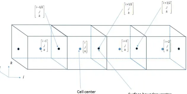
Figure II-1 shows a structured grid, with Cartesian coordinate convention. Eq. (II.13) is the discretized form of Eq. (II.12) that can be numerically solved.
1
n n t
V Q
Q Q F (II.13)
In Eq. (II.13), Qn is the conserved variables at a step time n while Qn1 is the conserved variables at step time n+1.
The calculation of the flux term of the conservative variables F
Q for the control surface encompassing the control volume represented here by a cell grid as given in Figure II-1.The calculation method is given in Eq. (II.14). HereFCi1/2and FVi1/ 2 are respectively the convective and viscous fluxes at the boundaries of the cell with a cell center coordinates
i j k, ,
T.The coordinates at the center of the boundaries in the 𝑖 direction are at coordinate
i1 2, ,j k
Tand
i1 2, ,j k
T. The 𝑗 and 𝑘 directions are treated in the same manner.17
1/2 1/2 1/ 2 1/2
1/2 1/2 1/ 2 1/2
1/2 1/2 1/2 1/2
1/2 1/2 1/2 1/2
1/ 2 1/2 1/ 2 1/2
1/ 2 1/2
C C
i i i i
C C
j j j j
C C
k j k j
V V
i i i i
V V
j j j j
V V
k j k
dS dS
dS dS
dS dS
dS dS
dS dS
dS
F Q F n F n
F n F n
F n F n
F n F n
F n F n
F n F
1/ 2ndSj1/2
(II.14)
Figure II-1 Coordinates at the center and surface boundaries
18
2.2. Second order central difference
The accuracy of a numerical scheme, in general depends of the applied approximations. In this research the viscous terms of the governing equations in Eq. (II.4) are discretized using the second order central differentiation scheme.
Let jbe the physical property at the cell-centered node to be approximated. Let jbe the cell average of the chosen physical property and the approximated value ofj, this is due to the use of the Finite Volume method that is basically applied to integral forms of conservative variables as shown in Eqs. (II.9), (II.10) and (II.11).
By replacing the integrand in Eq. (II.10) using the Taylor series expansion at the center of the cell we can write
1 2 3
1 2 3
2
2 2 3 3 2
1 2 3
1 , 1
2 2 2
1 1
2
x
x x
j j l l m
l l l m l m
x x x j j
d d d
V x x x
(II.15)Where h=
h1 h2 h3
T is the local Cartesian coordinate defining every point in the grid cell with its origin in the center and xi 2 hi xi 2
i1,2,3
and xithe dimension of the cell in each direction.The integration of Eq. (II.15) leads to the cancelation of the even order terms and the equation becomes
3 2
3 4
1 48 2
j j l
l l j
x x
h (II.16)And thus from Eq. (II.16), the difference between the average value of the cell and the cell center value is of second order.
2j j
h (II.17)
Eq. (II.17) explains the order of accuracy to which the estimated values of the viscous term
1/ 2 V
F i at the interface between two grid cells are achieved.
In upacs-LES, the viscous stress is calculated by Eq. (II.18) as for a Newtonian fluid.
19
τlm 2 S lm (II.18)
S𝑙𝑚 is the viscous strain-rate and it is defined by Eq. (II.19).
The dummy variables l, mand n take the values of the vectorsi j k, , defining the Cartesian base.
1 1
S 2 3
l m n
lm lm
m l n
u u u
x x x
(II.19)
For example, the flux in the 𝑖 direction for the grid cell with center coordinates
i j k, ,
T atthe boundary of coordinates
i1 2, ,j k
Tcan be calculated as in Eq. (II.20).2 1
3 ji ki
u u v w
x x y z
(II.20)
To calculate Eq. (II.20), it is necessary to estimate the gradient of each velocity components in each direction, this is done by simple central difference using the cell average velocities from the grid cells of coordinates
i j k, ,
Tand grid cell of coordinates
i1, ,j k
T.Eq. (II.21) is an example to estimate the derivative of the velocity u in the 𝑖 direction using the value of the velocities at the cell centers ui1 and ui with xi the distance between the two centers in the 𝑖 direction.
1 1/ 2
i i
i i
u u
x x
u
(II.21)
And similarly all the gradients are estimated following the same method shown here and named second order central difference.
20
2.3. Compact schemes
In Computational Aeroacoustics, there is a need to use numerical schemes leading to high accuracy results with low diffusion and dispersion errors and leading to good spectral resolution.
Several schemes satisfy these necessary requirements. Some of the widely used schemes by researches in this field are the high order compact schemes.
Kobayashi [24] formulated the high order compact schemes in finite volume method, and examined the stability, accuracy and spectral resolution of these methods.
Compact schemes are based on the Pade approximation of flux at the center of the boundary surfaces of the grid cell using the averaged values at the cell centers.
In this research, the implicit 6th order compact scheme is used for the calculation of the convective flux and only this case is explained hereafter, more details included in Appendix A, where the compact scheme is used to solve burgers equation.
For the implicit 6th order compact scheme, the interpolation of the value of a property at the interface of two grid cells with the index i1/ 2is done by the formula in Eq. (II.22).
In our research is any of the conservative variables in Eq. (II.2).
The average value at the adjacent grid cells in the line with j and k indexes fixed and
i
indexed as i1,i,i1and i2 are used to interpolate the values at the interface of the cells with indexes i1/ 2,i1/ 2and i3 / 2. The notation is shown in Figure II-2.
i6 1 1 i6 3 ii6 1 ii6 1 2
2 2 2
i i i i
i i i a b
(II.22)
The Pade interpolation method consists at finding the coefficients i6,aii6and bii6 by expanding the function with the Taylor series around the point of indexi1 / 2.
For the 6th-order compact scheme, this is achieved with the coefficients as in Eq. (II.23).
i6 ii6 ii6
1 29 1
, ,
3 a 36 b 36
(II.23)
As the Taylors series expansion assumes uniform spacing grid, the coefficients in Eq.
(II.23) can only be applied to uniform spacing grids.
21
Figure II-2 Example of grid and notation for inner points
Also, a 6th-order explicit compact scheme is applied for the points near the left boundary, which is given by the expression in Eq. (II.24).
1 ib6 1 0 ib6 2 1 ib6 3 2
2
a b c
(II.24)
where the averaged values of the cells in Figure II-3 are used.
Figure II-3 Example of grid and notation for left boundary
22
For the right boundary also the 6th-order explicit compact scheme is applied, which is given by the expression in Eq. (II.25).
1 ib6 ib6 ib 3
2
1 1 2 6 2
N N N N
N a N b c N
(II.25)
where the average values of the cells in Figure II-4 are used.
Figure II-4 Example of grid and notation for left boundary
High wavenumber numerical noise may be caused by the mesh non-uniformity as well as the discrete treatment of the boundary conditions. To suppress these unphysical cell-to-cell numerical oscillation, the low-pass filters in the form of Eq. (II.26) are used.
The compact filter is applied to the conservative variables in Eq. (II.2), where and * are the unfiltered and filtered cell-center variables, respectively.
The coefficients f and afj are given for different orders of accuracy as shown in Table II-1.
2
1 1
* * *
0 2
N i j i j
f i i f i fj
j
a
(II.26)In Eq. (II.26), N is the maximum order of the filter. However, in upacs-LES the order of the filter is gradually shifted from the maximum order inside the calculation domain to the 2nd order for the ghost cells near the boundary.
23 Table II-1 Coefficients of the compact Filter
order af0 af1 af2 af3 af4 af5 af
10th 193 126 256
f
105 302
256
f
15 30
64
f
45 90
512
f
5 10
256
f
1 2
512
f
0.48
8th 93 70
128
f
7 18
16
f
7 1 2
32
f
1 2
16
f
1 2
128
f
0.495
6th 11 10
16
f
15 34
32
f
3 1 2
16
f
1 2
32
f
0.4987
4th 5 6
8
f
1 2
2
f
1 2
8
f
0.4997
2nd 1 2
2
f
1 2 2
f
0.49992
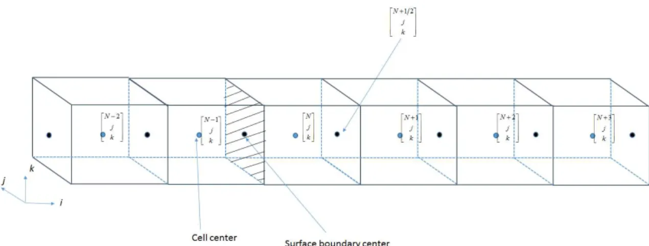
In this research, the 10th-order compact filter is the maximum order chosen. Therefore, in this case, the relationship between the boundary points and filter order is given by Figure II-5 and Figure II-6.
1 N
j k
N j k
Boundary surface
2 N
j k
3 N
j k
4 N
j k
5 N
j k
1 N
j k
2 N
j k
3 N
j k
4 N
j k
5 N
j k
*
N* 4
N* 3
N* 2
N* 1
N Figure II-5 Grid and notation for right boundary24 Figure II-6 Grid and notation for left boundary
1 j k
0
j k
Boundary surface
2 j k
3 j k
4
j k
5
j k
1
j k
2
j k
3
j k
4
j k
5
j k
*
0*
2*
3*
4*
125
2.4. Third-order Runge-Kutta time integration
The numerical simulations of turbulent flows with large eddy simulation require accurate and robust time-marching schemes. One of the prospective explicit time integration methods is given by the Runge-Kutta. These are high-order accuracy time integration methods by integration on different time stages. The Runge-Kutta methods are widely used in Computational Aeroacoustics.
The idea behind the Runge-Kutta method is to estimate the right-hand side in Eq. (II.14) on different stages using different value of conservative properties Qin an interval of time between n t and
n 1
t and to use all these values to estimate the value of Q at
n 1
t.In upacs-LES the third-order Runge-Kutta method is implemented. Such that the flux of conserved variables in Eq. (II.14) are function of Qas written in Eq. (II.27).
1
2 1 1
2
1
3
3 2
31 n
n
n
n n
t V t V t V
Q Q
Q Q F Q
Q Q F Q
Q Q F Q
(II.27)
with the coefficient specified as11 / 3,21 / 2 and 31


![Figure IV-10 Absorption coefficient for the tapered aperture 0.00.10.20.30.40.50.60.70.80.91.0200250300350400450 500 550 600 650 700Absorption coeffcientFrequency [Hz]](https://thumb-ap.123doks.com/thumbv2/123deta/9839864.1895420/66.918.158.801.657.1023/figure-iv-absorption-coefficient-tapered-aperture-absorption-coeffcientfrequency.webp)