Encoding Source Language with
Convolu5onal Neural Network for
Machine Transla5on
Fandong Meng, Zhengdong Lu, Mingxuan Wang,
Hang Li, Wenbin Jiang, Qun Liu,
ACL-‐IJCNLP 2015
すずかけ読み会
奥村・高村研究室博士二年
上垣外
英剛
概要
• 単語の分散表現に基づく統計的機械翻訳の
素性を提案
• 既存手法の
FFNNLM
に
CNN
と
Gate
を追加
•
dependency-‐to-‐stringデコーダにおいて既存
手法を上回る翻訳精度を達成
SMTのデコード
• 目的言語を一方向の順序で生成
日本語 を 英語 に 翻訳 する 事 は 難しい 。
デコードの問題点
•
NP困難問題
– 全ての候補列挙出来ない
• 近似探索
– 枝刈りのためのスコアが必要
• スコア
– 翻訳途中の情報で計算出来る事が望ましい
対数線形モデル
• スコアは対数線形モデルの形で表現される
事が多い
an example of HDR rule (b) for the top level
of (a), and an example of head rule (c). HDR
rules are constructed from head-dependents
re-lations. HDR rules can act as both translation
rules and reordering rules. And head rules are
used for translating source words.
We adopt the decoder proposed by Meng
et al. (2013) as a variant of Dep2Str
trans-lation that is easier to implement with
com-parable performance. Basically they extract
the HDR rules with GHKM (Galley et al.,
2004) algorithm. For the decoding procedure,
given a source dependency tree T , the
de-coder transverses T in post-order. The
bottom-up chart-based decoding algorithm with cube
pruning (Chiang, 2007; Huang and Chiang,
2007) is used to find the k-best items for each
node.
4.2 MT Decoder
Following Och and Ney (2002), we use a
gen-eral loglinear framework. Let d be a derivation
that convert a source dependency tree into a
tar-get string e. The probability of d is defined as:
P (d)
/
Y
i
i
(d)
i
(2)
where
i
are features defined on derivations
and
i
are the corresponding weights. Our
de-coder contains the following features:
Baseline Features:
• translation probabilities P (t|s) and
P (s
|t) of HDR rules;
• lexical translation probabilities P
LEX
(t|s)
and P
LEX
(s|t) of HDR rules;
• rule penalty exp( 1);
• pseudo translation rule penalty exp( 1);
• target word penalty exp(|e|);
• n-gram language model P
LM
(e);
Proposed Features:
• n-gram tagCNN joint language model
P
TLM
(e);
• n-gram inCNN joint language model
P
ILM
(e).
Our baseline decoder contains the first eight
features. The pseudo translation rule
(con-structed according to the word order of a HDR)
is to ensure the complete translation when no
matched rules is found during decoding. The
weights of all these features are tuned via
minimum error rate training (MERT) (Och,
2003). For the dependency-to-string decoder,
we set rule-threshold and stack-threshold to
10
3
, rule-limit to 100, stack-limit to 200.
5 Experiments
The experiments in this Section are designed to
answer the following questions:
1. Are our tagCNN and inCNN joint
lan-guage models able to improve translation
quality, and are they complementary to
each other?
2. Do inCNN and tagCNN benefit from
their guiding signal, compared to a
generic CNN?
3. For tagCNN, is it helpful to embed more
dependency structure, e.g., dependency
head of each affiliated word, as additional
information?
4. Can our gating strategy improve the
per-formance over max-pooling?
5.1 Setup
Data: Our training data are extracted from
LDC data
2
. We only keep the sentence pairs
that the length of source part no longer than
40 words, which covers over 90% of the
sen-tence. The bilingual training data consist of
221K sentence pairs, containing 5.0 million
Chinese words and 6.8 million English words.
The development set is NIST MT03 (795
tences) and test sets are MT04 (1499
sen-tences) and MT05 (917 sensen-tences) after
filter-ing with length limit.
Preprocessing: The word alignments are
ob-tained with GIZA++ (Och and Ney, 2003) on
the corpora in both directions, using the
“grow-diag-final-and” balance strategy (Koehn et al.,
2003). We adopt SRI Language Modeling
2
The corpora include LDC2002E18, LDC2003E07,
LDC2003E14, LDC2004T07, LDC2005T06.
25
今回はディープラーニングに基づいた素性を提案する話
翻訳が導出される確率 素性
先行研究
NNJM(Delvin et al., 2014)
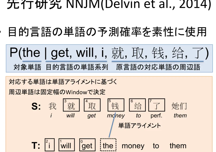
• 目的言語の単語の予測確率を素性に使用
Figure 1: Context vector for target word “the”, using a 3-word target history and a 5-word source window (i.e., n = 4 and m = 5). Here, “the” inherits its affiliation from “money” because this is the first aligned word to its right. The number in each box denotes the index of the word in the context vector. This indexing must be consistent across samples, but the absolute ordering does not affect results.
128.3 At every epoch, which we define as 20,000 minibatches, the likelihood of a validation set is computed. If this likelihood is worse than the pre-vious epoch, the learning rate is multiplied by 0.5. The training is run for 40 epochs. The training data ranges from 10-30M words, depending on the condition. We perform a basic weight update with no L2 regularization or momentum. However, we have found it beneficial to clip each weight update to the range of [-0.1, 0.1], to prevent the training from entering degenerate search spaces (Pascanu et al., 2012).
Training is performed on a single Tesla K10 GPU, with each epoch (128*20k = 2.6M samples) taking roughly 1100 seconds to run, resulting in a total training time of ⇠12 hours. Decoding is performed on a CPU.
2.3 Self-Normalized Neural Network
The computational cost of NNLMs is a significant issue in decoding, and this cost is dominated by the output softmax over the entire target vocabu-lary. Even class-based approaches such as Le et al. (2012) require a 2-20k shortlist vocabulary, and are therefore still quite costly.
Here, our goal is to be able to use a fairly large vocabulary without word classes, and to sim-ply avoid computing the entire output layer at de-code time.4 To do this, we present the novel technique of self-normalization, where the output layer scores are close to being probabilities with-out explicitly performing a softmax.
Formally, we define the standard softmax log
3We do not divide the gradient by the minibatch size. For
those who do, this is equivalent to using an initial learning rate of 10 3
⇤ 128 ⇡ 10 1.
4We are not concerned with speeding up training time, as
we already find GPU training time to be adequate.
likelihood as: log(P (x)) = log eUr(x) Z(x) ! = Ur(x) log(Z(x)) Z(x) = ⌃|V |r0=1eUr0(x)
where x is the sample, U is the raw output layer scores, r is the output layer row corresponding to the observed target word, and Z(x) is the softmax normalizer.
If we could guarantee that log(Z(x)) were al-ways equal to 0 (i.e., Z(x) = 1) then at decode time we would only have to compute row r of the output layer instead of the whole matrix. While we cannot train a neural network with this guaran-tee, we can explicitly encourage the log-softmax normalizer to be as close to 0 as possible by aug-menting our training objective function:
L = X i ⇥ log(P (xi)) ↵(log(Z(xi)) 0)2⇤ = X i ⇥ log(P (xi)) ↵ log2(Z(xi))⇤
In this case, the output layer bias weights are initialized to log(1/|V |), so that the initial net-work is self-normalized. At decode time, we sim-ply use Ur(x) as the feature score, rather than
log(P (x)). For our NNJM architecture, self-normalization increases the lookup speed during decoding by a factor of ⇠15x.
Table 1 shows the neural network training re-sults with various values of the free parameter ↵. In all subsequent MT experiments, we use ↵ = 10 1.
We should note that Vaswani et al. (2013) im-plements a method called Noise Contrastive Es-timation (NCE) that is also used to train self-normalized NNLMs. Although NCE results in faster training time, it has the downside that there 1372
Figure 1: Context vector for target word “the”, using a 3-word target history and a 5-word source window (i.e., n = 4 and m = 5). Here, “the” inherits its affiliation from “money” because this is the first aligned word to its right. The number in each box denotes the index of the word in the context vector. This indexing must be consistent across samples, but the absolute ordering does not affect results.
128.3 At every epoch, which we define as 20,000 minibatches, the likelihood of a validation set is computed. If this likelihood is worse than the pre-vious epoch, the learning rate is multiplied by 0.5. The training is run for 40 epochs. The training data ranges from 10-30M words, depending on the condition. We perform a basic weight update with no L2 regularization or momentum. However, we have found it beneficial to clip each weight update to the range of [-0.1, 0.1], to prevent the training from entering degenerate search spaces (Pascanu et al., 2012).
Training is performed on a single Tesla K10 GPU, with each epoch (128*20k = 2.6M samples) taking roughly 1100 seconds to run, resulting in a total training time of ⇠12 hours. Decoding is performed on a CPU.
2.3 Self-Normalized Neural Network
The computational cost of NNLMs is a significant issue in decoding, and this cost is dominated by the output softmax over the entire target vocabu-lary. Even class-based approaches such as Le et al. (2012) require a 2-20k shortlist vocabulary, and are therefore still quite costly.
Here, our goal is to be able to use a fairly large vocabulary without word classes, and to sim-ply avoid computing the entire output layer at de-code time.4 To do this, we present the novel technique of self-normalization, where the output layer scores are close to being probabilities with-out explicitly performing a softmax.
Formally, we define the standard softmax log
3We do not divide the gradient by the minibatch size. For
those who do, this is equivalent to using an initial learning rate of 10 3
⇤ 128 ⇡ 10 1.
4We are not concerned with speeding up training time, as
we already find GPU training time to be adequate.
likelihood as: log(P (x)) = log eUr(x) Z(x) ! = Ur(x) log(Z(x)) Z(x) = ⌃|V |r0=1eUr0(x)
where x is the sample, U is the raw output layer scores, r is the output layer row corresponding to the observed target word, and Z(x) is the softmax normalizer.
If we could guarantee that log(Z(x)) were al-ways equal to 0 (i.e., Z(x) = 1) then at decode time we would only have to compute row r of the output layer instead of the whole matrix. While we cannot train a neural network with this guaran-tee, we can explicitly encourage the log-softmax normalizer to be as close to 0 as possible by aug-menting our training objective function:
L = X i ⇥ log(P (xi)) ↵(log(Z(xi)) 0)2⇤ = X i ⇥ log(P (xi)) ↵ log2(Z(xi))⇤
In this case, the output layer bias weights are initialized to log(1/|V |), so that the initial net-work is self-normalized. At decode time, we sim-ply use Ur(x) as the feature score, rather than
log(P (x)). For our NNJM architecture, self-normalization increases the lookup speed during decoding by a factor of ⇠15x.
Table 1 shows the neural network training re-sults with various values of the free parameter ↵. In all subsequent MT experiments, we use ↵ = 10 1.
We should note that Vaswani et al. (2013) im-plements a method called Noise Contrastive Es-timation (NCE) that is also used to train self-normalized NNLMs. Although NCE results in faster training time, it has the downside that there
1372
Figure 1: Context vector for target word “the”, using a 3-word target history and a 5-word source window
(i.e., n = 4 and m = 5). Here, “the” inherits its affiliation from “money” because this is the first aligned
word to its right. The number in each box denotes the index of the word in the context vector. This
indexing must be consistent across samples, but the absolute ordering does not affect results.
128.
3At every epoch, which we define as 20,000
minibatches, the likelihood of a validation set is
computed. If this likelihood is worse than the
pre-vious epoch, the learning rate is multiplied by 0.5.
The training is run for 40 epochs. The training
data ranges from 10-30M words, depending on the
condition. We perform a basic weight update with
no L2 regularization or momentum. However, we
have found it beneficial to clip each weight update
to the range of [-0.1, 0.1], to prevent the training
from entering degenerate search spaces (Pascanu
et al., 2012).
Training is performed on a single Tesla K10
GPU, with each epoch (128*20k = 2.6M samples)
taking roughly 1100 seconds to run, resulting in
a total training time of ⇠12 hours. Decoding is
performed on a CPU.
2.3 Self-Normalized Neural Network
The computational cost of NNLMs is a significant
issue in decoding, and this cost is dominated by
the output softmax over the entire target
vocabu-lary. Even class-based approaches such as Le et
al. (2012) require a 2-20k shortlist vocabulary, and
are therefore still quite costly.
Here, our goal is to be able to use a fairly
large vocabulary without word classes, and to
sim-ply avoid computing the entire output layer at
de-code time.
4To do this, we present the novel
technique of self-normalization, where the output
layer scores are close to being probabilities
with-out explicitly performing a softmax.
Formally, we define the standard softmax log
3
We do not divide the gradient by the minibatch size. For
those who do, this is equivalent to using an initial learning
rate of 10
3⇤ 128 ⇡ 10
1.
4
We are not concerned with speeding up training time, as
we already find GPU training time to be adequate.
likelihood as:
log(P (x)) = log
e
Ur(x)Z(x)
!
= U
r(x) log(Z(x))
Z(x) = ⌃
|V |r0=1e
Ur0(x)where x is the sample, U is the raw output layer
scores, r is the output layer row corresponding to
the observed target word, and Z(x) is the softmax
normalizer.
If we could guarantee that log(Z(x)) were
al-ways equal to 0 (i.e., Z(x) = 1) then at decode
time we would only have to compute row r of the
output layer instead of the whole matrix. While
we cannot train a neural network with this
guaran-tee, we can explicitly encourage the log-softmax
normalizer to be as close to 0 as possible by
aug-menting our training objective function:
L =
X
i⇥
log(P (x
i)) ↵(log(Z(x
i)) 0)
2⇤
=
X
i⇥
log(P (x
i)) ↵ log
2(Z(x
i))
⇤
In this case, the output layer bias weights are
initialized to log(1/|V |), so that the initial
net-work is self-normalized. At decode time, we
sim-ply use U
r(x) as the feature score, rather than
log(P (x)). For our NNJM architecture,
self-normalization increases the lookup speed during
decoding by a factor of ⇠15x.
Table 1 shows the neural network training
re-sults with various values of the free parameter
↵
. In all subsequent MT experiments, we use
↵ = 10
1.
We should note that Vaswani et al. (2013)
im-plements a method called Noise Contrastive
Es-timation (NCE) that is also used to train
self-normalized NNLMs. Although NCE results in
faster training time, it has the downside that there
1372
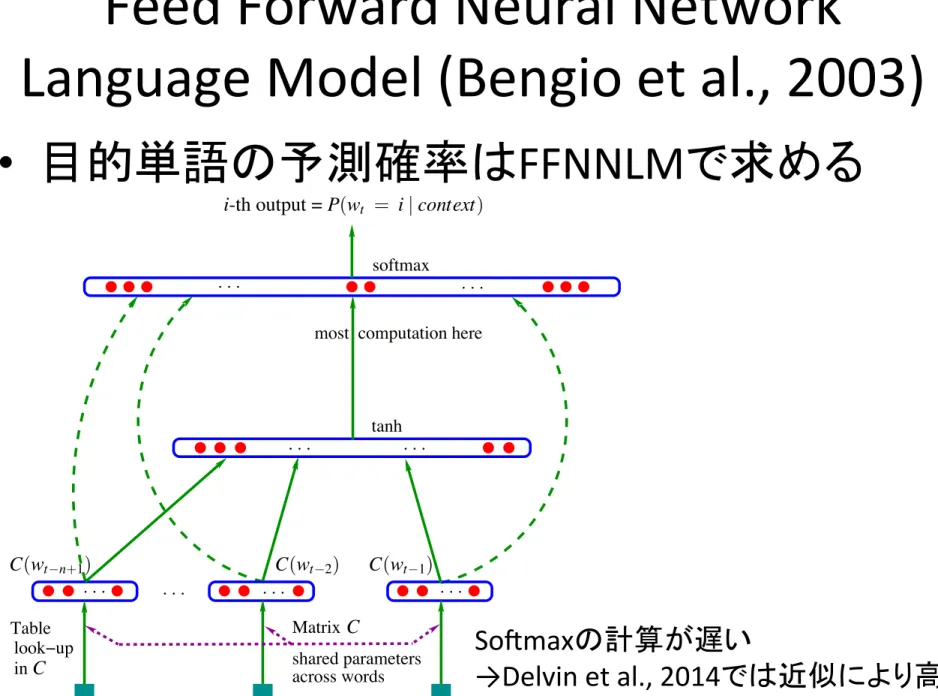
原言語の対応単語の周辺語 目的言語の単語系列 単語アライメント 対象単語 対応する単語は単語アライメントに基づく 周辺単語は固定幅のWindowで決定Feed Forward Neural Network
Language Model (Bengio et al., 2003)
• 目的単語の予測確率は
FFNNLMで求める
BENGIO, DUCHARME, VINCENT AND JAUVIN
softmax tanh . . . . . . . . . . . . . . . across words
most computation here
index for index for index for shared parameters Matrix in look−up Table . . . C C wt 1 wt 2 C(wt 2) C(wt 1) C(wt n+1) wt n+1
i-th output = P(wt = i | context)
Figure 1: Neural architecture: f (i, wt 1,··· ,wt n+1) = g(i,C(wt 1),··· ,C(wt n+1)) where g is the neural network and C(i) is the i-th word feature vector.
parameters of the mapping C are simply the feature vectors themselves, represented by a |V | ⇥ m matrix C whose row i is the feature vector C(i) for word i. The function g may be implemented by a feed-forward or recurrent neural network or another parametrized function, with parameters ω. The overall parameter set is θ = (C, ω).
Training is achieved by looking for θ that maximizes the training corpus penalized log-likelihood:
L = 1
T
∑
t log f (wt, wt 1,··· ,wt n+1; θ) + R(θ),where R(θ) is a regularization term. For example, in our experiments, R is a weight decay penalty applied only to the weights of the neural network and to the C matrix, not to the biases.3
In the above model, the number of free parameters only scales linearly with V , the number of words in the vocabulary. It also only scales linearly with the order n : the scaling factor could be reduced to sub-linear if more sharing structure were introduced, e.g. using a time-delay neural network or a recurrent neural network (or a combination of both).
In most experiments below, the neural network has one hidden layer beyond the word features mapping, and optionally, direct connections from the word features to the output. Therefore there are really two hidden layers: the shared word features layer C, which has no non-linearity (it would not add anything useful), and the ordinary hyperbolic tangent hidden layer. More precisely, the neural network computes the following function, with a softmax output layer, which guarantees positive probabilities summing to 1:
ˆ
P(wt|wt 1,··· wt n+1) = e ywt ∑ieyi
.
3. The biases are the additive parameters of the neural network, such as b and d in equation 1 below.
1142
SoXmaxの計算が遅い
今回の手法
• 既存手法に
CNN
と
Gate
を追加
• 固定幅の
Context Windowを使用しない
• 手法は二種類
–
tagCNN
–
inCNN
tagCNN
(a) tagCNN (b) inCNN
Figure 1: Illustration for joint LM based on CNN encoder. RoadMap: In the remainder of this paper,
we start with a brief overview of joint language model in Section 2, while the convolutional en-coders, as the key component of which, will be described in detail in Section 3. Then in Sec-tion 4 we discuss the decoding algorithm with the proposed models. The experiment results are reported in Section 5, followed by Section 6 and 7 for related work and conclusion.
2 Joint Language Model
Our joint model with CNN encoders can be il-lustrated in Figure 1 (a) & (b), which consists 1) a CNN encoder, namely tagCNN or inCNN, to represent the information in the source sen-tences, and 2) an NN-based model for predict-ing the next words, with representations from CNN encoders and the history words in target sentence as inputs.
In the joint language model, the
probabil-ity of the target word en, given previous k
target words {en k,· · ·, en 1} and the
repre-sentations from CNN-encoders for source sen-tence S are
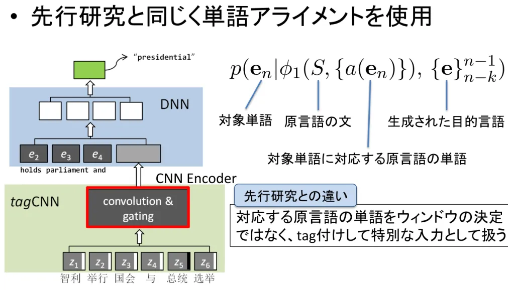
tagCNN: p(en| 1(S, {a(en)}), {e}n 1n k)
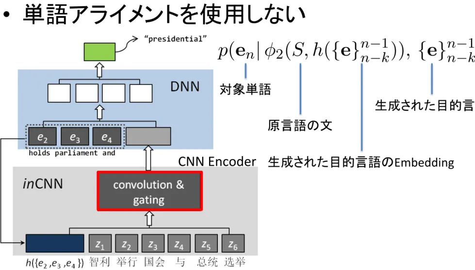
inCNN: p(en| 2(S, h({e}n 1n k)), {e}n 1n k),
where 1(S, {a(en)}) stands for the
represen-tation given by tagCNN with the set of indexes {a(en)} of source words aligned to the target
word en, and 2(S, h({e}n 1n k)) stands for the
representation from inCNN with the attention
signal h({e}n 1
n k).
Let us use the example in Figure 1, where the task is to translate the Chinese sentence
into English. In evaluating a target
lan-guage sequence “holds parliament
and presidential”, with “holds
parliament and” as the proceeding words (assume 4-gram LM), and the affiliated
source word1 of “presidential” being
“Zˇongtˇong” (determined by word
align-ment), tagCNN generates 1(S, {4}) (the
in-dex of “Zˇongtˇong” is 4), and inCNN
gener-ates 2(S, h(holds parliament and)).
The DNN component then takes
"holds parliament and" and
( 1 or 2) as input to give the
con-ditional probability for next word, e.g., p("presidential"| 1|2, {holds,
parliament, and}).
3 Convolutional Models
We start with the generic architecture for convolutional encoder, and then proceed to
tagCNN and inCNN as two extensions.
1For an aligned target word, we take its aligned source words as its affiliated source words. And for an unaligned word, we inherit its affiliation from the closest aligned word, with preference given to the right (Devlin et al., 2014). Since the word alignment is of many-to-many, one target word may has multi affiliated source words.
21
(a) tagCNN
(b) inCNN
Figure 1: Illustration for joint LM based on CNN encoder.
RoadMap: In the remainder of this paper,
we start with a brief overview of joint language
model in Section 2, while the convolutional
en-coders, as the key component of which, will be
described in detail in Section 3. Then in
Sec-tion 4 we discuss the decoding algorithm with
the proposed models. The experiment results
are reported in Section 5, followed by Section 6
and 7 for related work and conclusion.
2 Joint Language Model
Our joint model with CNN encoders can be
il-lustrated in Figure 1 (a) & (b), which consists
1) a CNN encoder, namely tagCNN or inCNN,
to represent the information in the source
sen-tences, and 2) an NN-based model for
predict-ing the next words, with representations from
CNN encoders and the history words in target
sentence as inputs.
In the joint language model, the
probabil-ity of the target word e
n, given previous k
target words {e
n k,
· · ·, e
n 1} and the
repre-sentations from CNN-encoders for source
sen-tence S are
tag
CNN: p(e
n|
1(S, {a(e
n)}), {e}
n 1n k)
inCNN: p(e
n|
2(S, h({e}
n 1n k
)), {e}
n 1n k),
where
1(S, {a(e
n)}) stands for the
represen-tation given by tagCNN with the set of indexes
{a(e
n)} of source words aligned to the target
word e
n, and
2(S, h({e}
n 1n k
)) stands for the
representation from inCNN with the attention
signal h({e}
n 1n k
).
Let us use the example in Figure 1, where
the task is to translate the Chinese sentence
into English.
In evaluating a target
lan-guage
sequence
“holds parliament
and presidential
”,
with
“holds
parliament and
” as the proceeding
words (assume 4-gram LM), and the affiliated
source word
1of “presidential” being
“Zˇ
ongtˇ
ong
” (determined by word
align-ment), tagCNN generates
1(S, {4}) (the
in-dex of “Zˇ
ongtˇ
ong
” is 4), and inCNN
gener-ates
2(S, h(holds parliament and)).
The
DNN
component
then
takes
"holds parliament and"
and
(
1or
2) as input to give the
con-ditional probability for next word, e.g.,
p("presidential"
|
1|2,
{holds,
parliament, and}).
3 Convolutional Models
We start with the generic architecture for
convolutional encoder, and then proceed to
tag
CNN and inCNN as two extensions.
1
For an aligned target word, we take its aligned source
words as its affiliated source words. And for an unaligned
word, we inherit its affiliation from the closest aligned
word, with preference given to the right (Devlin et al.,
2014). Since the word alignment is of many-to-many,
one target word may has multi affiliated source words.
21
• 先行研究と同じく単語アライメントを使用
対象単語 原言語の文 生成された目的言語 対象単語に対応する原言語の単語 対応する原言語の単語をウィンドウの決定 ではなく、tag付けして特別な入力として扱う 先行研究との違い CNN EncoderinCNN
(a) tagCNN (b) inCNN
Figure 1: Illustration for joint LM based on CNN encoder. RoadMap: In the remainder of this paper,
we start with a brief overview of joint language model in Section 2, while the convolutional en-coders, as the key component of which, will be described in detail in Section 3. Then in Sec-tion 4 we discuss the decoding algorithm with the proposed models. The experiment results are reported in Section 5, followed by Section 6 and 7 for related work and conclusion.
2 Joint Language Model
Our joint model with CNN encoders can be il-lustrated in Figure 1 (a) & (b), which consists 1) a CNN encoder, namely tagCNN or inCNN, to represent the information in the source sen-tences, and 2) an NN-based model for predict-ing the next words, with representations from CNN encoders and the history words in target sentence as inputs.
In the joint language model, the probabil-ity of the target word en, given previous k target words {en k,· · ·, en 1} and the repre-sentations from CNN-encoders for source sen-tence S are
tagCNN: p(en| 1(S, {a(en)}), {e}n 1n k) inCNN: p(en| 2(S, h({e}n 1n k)), {e}n 1n k), where 1(S, {a(en)}) stands for the represen-tation given by tagCNN with the set of indexes {a(en)} of source words aligned to the target word en, and 2(S, h({e}n 1n k)) stands for the representation from inCNN with the attention
signal h({e}n 1 n k).
Let us use the example in Figure 1, where the task is to translate the Chinese sentence
into English. In evaluating a target lan-guage sequence “holds parliament and presidential”, with “holds parliament and” as the proceeding words (assume 4-gram LM), and the affiliated source word1 of “presidential” being “Zˇongtˇong” (determined by word align-ment), tagCNN generates 1(S, {4}) (the in-dex of “Zˇongtˇong” is 4), and inCNN gener-ates 2(S, h(holds parliament and)).
The DNN component then takes
"holds parliament and" and ( 1 or 2) as input to give the con-ditional probability for next word, e.g., p("presidential"| 1|2, {holds,
parliament, and}).
3 Convolutional Models
We start with the generic architecture for convolutional encoder, and then proceed to tagCNN and inCNN as two extensions.
1For an aligned target word, we take its aligned source
words as its affiliated source words. And for an unaligned word, we inherit its affiliation from the closest aligned word, with preference given to the right (Devlin et al., 2014). Since the word alignment is of many-to-many, one target word may has multi affiliated source words.
21
• 単語アライメントを使用しない
(a) tagCNN
(b) inCNN
Figure 1: Illustration for joint LM based on CNN encoder.
RoadMap: In the remainder of this paper,
we start with a brief overview of joint language
model in Section 2, while the convolutional
en-coders, as the key component of which, will be
described in detail in Section 3. Then in
Sec-tion 4 we discuss the decoding algorithm with
the proposed models. The experiment results
are reported in Section 5, followed by Section 6
and 7 for related work and conclusion.
2 Joint Language Model
Our joint model with CNN encoders can be
il-lustrated in Figure 1 (a) & (b), which consists
1) a CNN encoder, namely tagCNN or inCNN,
to represent the information in the source
sen-tences, and 2) an NN-based model for
predict-ing the next words, with representations from
CNN encoders and the history words in target
sentence as inputs.
In the joint language model, the
probabil-ity of the target word e
n, given previous k
target words {e
n k,
· · ·, e
n 1} and the
repre-sentations from CNN-encoders for source
sen-tence S are
tagCNN: p(e
n|
1(S, {a(e
n)}), {e}
n 1n k)
inCNN: p(e
n|
2(S, h({e}
n 1n k)), {e}
n 1n k),
where
1(S, {a(e
n)}) stands for the
represen-tation given by tagCNN with the set of indexes
{a(e
n)} of source words aligned to the target
word e
n, and
2(S, h({e}
n 1n k)) stands for the
representation from inCNN with the attention
signal h({e}
n 1 n k).
Let us use the example in Figure 1, where
the task is to translate the Chinese sentence
into English.
In evaluating a target
lan-guage
sequence
“holds parliament
and presidential
”,
with
“holds
parliament and” as the proceeding
words (assume 4-gram LM), and the affiliated
source word
1of “presidential” being
“Zˇongtˇong” (determined by word
align-ment), tagCNN generates
1(S, {4}) (the
in-dex of “Zˇongtˇong” is 4), and inCNN
gener-ates
2(S, h(holds parliament and)).
The
DNN
component
then
takes
"holds parliament and"
and
(
1or
2) as input to give the
con-ditional probability for next word, e.g.,
p("presidential"
|
1|2,
{holds,
parliament, and}).
3 Convolutional Models
We start with the generic architecture for
convolutional encoder, and then proceed to
tagCNN and inCNN as two extensions.
1For an aligned target word, we take its aligned source
words as its affiliated source words. And for an unaligned word, we inherit its affiliation from the closest aligned word, with preference given to the right (Devlin et al., 2014). Since the word alignment is of many-to-many, one target word may has multi affiliated source words.
21
生成された目的言語のEmbedding 対象単語 原言語の文 生成された目的言語 CNN EncoderCNN Encoder
Figure 2: Illustration for the CNN encoders.
3.1 Generic CNN Encoder
The basic architecture is of a generic CNN
en-coder is illustrated in Figure 2 (a), which has a
fixed architecture consisting of six layers:
Layer-0: the input layer, which takes words
in the form of embedding vectors. In our
work, we set the maximum length of
sen-tences to 40 words. For sensen-tences shorter
than that, we put zero padding at the
be-ginning of sentences.
Layer-1: a convolution layer after Layer-0,
with window size = 3. As will be
dis-cussed in Section 3.2 and 3.3, the
guid-ing signal are injected into this layer for
“guided version”.
2: a local gating layer after
Layer-1, which simply takes a weighted sum
over feature-maps in non-adjacent
win-dow with size = 2.
Layer-3: a convolution layer after Layer-2, we
perform another convolution with window
size = 3.
Layer-4: we perform a global gating over
feature-maps on Layer-3.
Layer-5: fully connected weights that maps
the output of Layer-4 to this layer as the
final representation.
3.1.1 Convolution
As shown in Figure 2 (a), the convolution in
Layer-1 operates on sliding windows of words
(width k
1), and the similar definition of
win-dows carries over to higher layers. Formally,
for source sentence input x = {x
1,
· · · , x
N},
the convolution unit for feature map of type-f
(among F
`of them) on Layer-` is
z
i(`,f )(x) = (w
(`,f )ˆz
(` 1)i+ b
(`,f )),
` = 1, 3,
f = 1, 2,
· · · , F
`(1)
where
• z
i(`,f )(x) gives the output of feature map
of type-f for location i in Layer-`;
• w
(`,f )is the parameters for f on Layer-`;
• (·) is the Sigmoid activation function;
• ˆz
(` 1)idenotes the segment of Layer-` 1
for the convolution at location i , while
ˆz
(0)i def= [x
>i
, x
>i+1, x
>i+2]
>concatenates the vectors for 3 words from
sentence input x.
3.1.2 Gating
Previous CNNs, including those for NLP
tasks (Hu et al., 2014; Kalchbrenner et al.,
2014), take a straightforward
convolution-pooling strategy, in which the “fusion”
deci-sions (e.g., selecting the largest one in
max-pooling) are based on the values of
feature-maps. This is essentially a soft template
match-ing, which works for tasks like classification,
but harmful for keeping the composition
func-tionality of convolution, which is critical for
modeling sentences. In this paper, we propose
to use separate gating unit to release the score
function duty from the convolution, and let it
focus on composition.
22
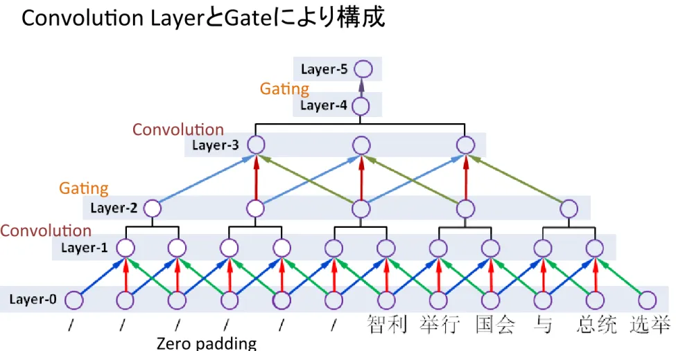
Convolu5on Ga5ng Convolu5on Ga5ng Zero padding 入力単語は40単語で固定Convolu5on LayerとGateにより構成
CNN Encoder
Figure 2: Illustration for the CNN encoders.
3.1 Generic CNN Encoder
The basic architecture is of a generic CNN
en-coder is illustrated in Figure 2 (a), which has a
fixed architecture consisting of six layers:
Layer-0: the input layer, which takes words
in the form of embedding vectors. In our
work, we set the maximum length of
sen-tences to 40 words. For sensen-tences shorter
than that, we put zero padding at the
be-ginning of sentences.
Layer-1: a convolution layer after Layer-0,
with window size = 3. As will be
dis-cussed in Section 3.2 and 3.3, the
guid-ing signal are injected into this layer for
“guided version”.
2: a local gating layer after
Layer-1, which simply takes a weighted sum
over feature-maps in non-adjacent
win-dow with size = 2.
Layer-3: a convolution layer after Layer-2, we
perform another convolution with window
size = 3.
Layer-4: we perform a global gating over
feature-maps on Layer-3.
Layer-5: fully connected weights that maps
the output of Layer-4 to this layer as the
final representation.
3.1.1 Convolution
As shown in Figure 2 (a), the convolution in
Layer-1 operates on sliding windows of words
(width k
1), and the similar definition of
win-dows carries over to higher layers. Formally,
for source sentence input x = {x
1,
· · · , x
N},
the convolution unit for feature map of type-f
(among F
`of them) on Layer-` is
z
i(`,f )(x) = (w
(`,f )ˆz
(` 1)i+ b
(`,f )),
` = 1, 3,
f = 1, 2,
· · · , F
`(1)
where
• z
i(`,f )(x) gives the output of feature map
of type-f for location i in Layer-`;
• w
(`,f )is the parameters for f on Layer-`;
• (·) is the Sigmoid activation function;
• ˆz
(` 1)idenotes the segment of Layer-` 1
for the convolution at location i , while
ˆz
(0)i def= [x
>i
, x
>i+1, x
>i+2]
>concatenates the vectors for 3 words from
sentence input x.
3.1.2 Gating
Previous CNNs, including those for NLP
tasks (Hu et al., 2014; Kalchbrenner et al.,
2014), take a straightforward
convolution-pooling strategy, in which the “fusion”
deci-sions (e.g., selecting the largest one in
max-pooling) are based on the values of
feature-maps. This is essentially a soft template
match-ing, which works for tasks like classification,
but harmful for keeping the composition
func-tionality of convolution, which is critical for
modeling sentences. In this paper, we propose
to use separate gating unit to release the score
function duty from the convolution, and let it
focus on composition.
22
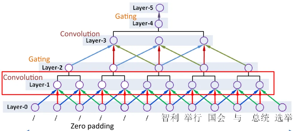
Convolu5on Ga5ng Convolu5on Ga5ng Zero padding 入力単語は40単語で固定Convolu5onとGateにより構成
Layer 1
•
Window size 3
•
Layer 0 から入力されたベクトルを畳み込む
–
Layer 0 は word embeddingを行う
• シグモイド関数を活性化関数として使用
CNN Encoder
Figure 2: Illustration for the CNN encoders.
3.1 Generic CNN Encoder
The basic architecture is of a generic CNN
en-coder is illustrated in Figure 2 (a), which has a
fixed architecture consisting of six layers:
Layer-0: the input layer, which takes words
in the form of embedding vectors. In our
work, we set the maximum length of
sen-tences to 40 words. For sensen-tences shorter
than that, we put zero padding at the
be-ginning of sentences.
Layer-1: a convolution layer after Layer-0,
with window size = 3. As will be
dis-cussed in Section 3.2 and 3.3, the
guid-ing signal are injected into this layer for
“guided version”.
2: a local gating layer after
Layer-1, which simply takes a weighted sum
over feature-maps in non-adjacent
win-dow with size = 2.
Layer-3: a convolution layer after Layer-2, we
perform another convolution with window
size = 3.
Layer-4: we perform a global gating over
feature-maps on Layer-3.
Layer-5: fully connected weights that maps
the output of Layer-4 to this layer as the
final representation.
3.1.1 Convolution
As shown in Figure 2 (a), the convolution in
Layer-1 operates on sliding windows of words
(width k
1), and the similar definition of
win-dows carries over to higher layers. Formally,
for source sentence input x = {x
1,
· · · , x
N},
the convolution unit for feature map of type-f
(among F
`of them) on Layer-` is
z
i(`,f )(x) = (w
(`,f )ˆz
(` 1)i+ b
(`,f )),
` = 1, 3,
f = 1, 2,
· · · , F
`(1)
where
• z
i(`,f )(x) gives the output of feature map
of type-f for location i in Layer-`;
• w
(`,f )is the parameters for f on Layer-`;
• (·) is the Sigmoid activation function;
• ˆz
(` 1)idenotes the segment of Layer-` 1
for the convolution at location i , while
ˆz
(0)i def= [x
>i
, x
>i+1, x
>i+2]
>concatenates the vectors for 3 words from
sentence input x.
3.1.2 Gating
Previous CNNs, including those for NLP
tasks (Hu et al., 2014; Kalchbrenner et al.,
2014), take a straightforward
convolution-pooling strategy, in which the “fusion”
deci-sions (e.g., selecting the largest one in
max-pooling) are based on the values of
feature-maps. This is essentially a soft template
match-ing, which works for tasks like classification,
but harmful for keeping the composition
func-tionality of convolution, which is critical for
modeling sentences. In this paper, we propose
to use separate gating unit to release the score
function duty from the convolution, and let it
focus on composition.
22
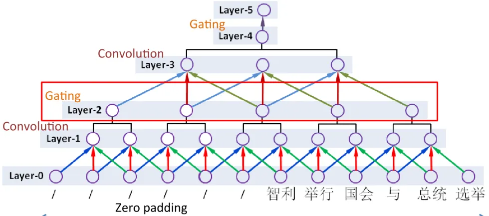
Convolu5on Ga5ng Convolu5on Ga5ng Zero padding 入力単語は40単語で固定Convolu5onとGateにより構成
Layer 2
•
Window size 2 の Gate
•
Layer 1 から入力されたベクトルの加重和を出
力
3 4 5 6
(3, 4, 5) (4, 5, 6) (3, 4, 5, 6)
CNN Encoder
Figure 2: Illustration for the CNN encoders.
3.1 Generic CNN Encoder
The basic architecture is of a generic CNN
en-coder is illustrated in Figure 2 (a), which has a
fixed architecture consisting of six layers:
Layer-0: the input layer, which takes words
in the form of embedding vectors. In our
work, we set the maximum length of
sen-tences to 40 words. For sensen-tences shorter
than that, we put zero padding at the
be-ginning of sentences.
Layer-1: a convolution layer after Layer-0,
with window size = 3. As will be
dis-cussed in Section 3.2 and 3.3, the
guid-ing signal are injected into this layer for
“guided version”.
2: a local gating layer after
Layer-1, which simply takes a weighted sum
over feature-maps in non-adjacent
win-dow with size = 2.
Layer-3: a convolution layer after Layer-2, we
perform another convolution with window
size = 3.
Layer-4: we perform a global gating over
feature-maps on Layer-3.
Layer-5: fully connected weights that maps
the output of Layer-4 to this layer as the
final representation.
3.1.1 Convolution
As shown in Figure 2 (a), the convolution in
Layer-1 operates on sliding windows of words
(width k
1), and the similar definition of
win-dows carries over to higher layers. Formally,
for source sentence input x = {x
1,
· · · , x
N},
the convolution unit for feature map of type-f
(among F
`of them) on Layer-` is
z
i(`,f )(x) = (w
(`,f )ˆz
(` 1)i+ b
(`,f )),
` = 1, 3,
f = 1, 2,
· · · , F
`(1)
where
• z
i(`,f )(x) gives the output of feature map
of type-f for location i in Layer-`;
• w
(`,f )is the parameters for f on Layer-`;
• (·) is the Sigmoid activation function;
• ˆz
(` 1)idenotes the segment of Layer-` 1
for the convolution at location i , while
ˆz
(0)i def= [x
>i
, x
>i+1, x
>i+2]
>concatenates the vectors for 3 words from
sentence input x.
3.1.2 Gating
Previous CNNs, including those for NLP
tasks (Hu et al., 2014; Kalchbrenner et al.,
2014), take a straightforward
convolution-pooling strategy, in which the “fusion”
deci-sions (e.g., selecting the largest one in
max-pooling) are based on the values of
feature-maps. This is essentially a soft template
match-ing, which works for tasks like classification,
but harmful for keeping the composition
func-tionality of convolution, which is critical for
modeling sentences. In this paper, we propose
to use separate gating unit to release the score
function duty from the convolution, and let it
focus on composition.
22
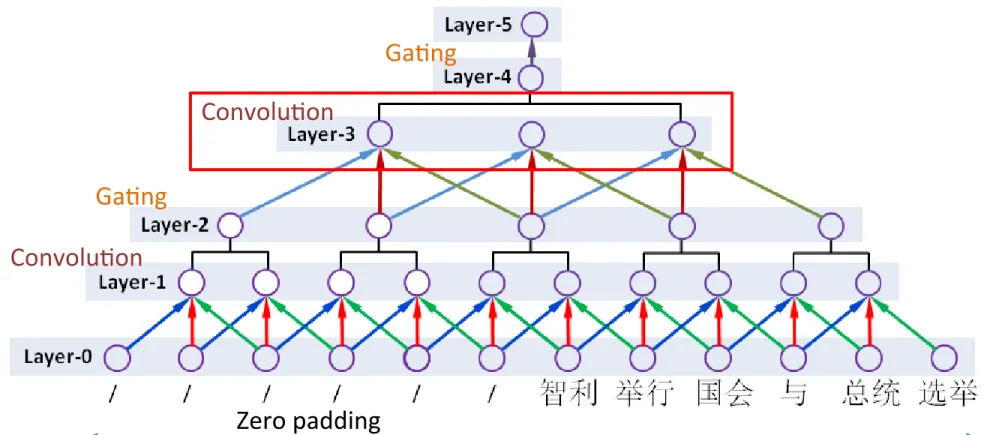
Convolu5on Ga5ng Convolu5on Ga5ng Zero padding 入力単語は40単語で固定Convolu5onとGateにより構成
Layer-‐3
•
Layer 2の出力に対して畳み込みを行う
Convolu5on & ga5ng
Figure 2: Illustration for the CNN encoders.
3.1 Generic CNN Encoder
The basic architecture is of a generic CNN
en-coder is illustrated in Figure 2 (a), which has a
fixed architecture consisting of six layers:
Layer-0: the input layer, which takes words
in the form of embedding vectors. In our
work, we set the maximum length of
sen-tences to 40 words. For sensen-tences shorter
than that, we put zero padding at the
be-ginning of sentences.
Layer-1: a convolution layer after Layer-0,
with window size = 3. As will be
dis-cussed in Section 3.2 and 3.3, the
guid-ing signal are injected into this layer for
“guided version”.
2: a local gating layer after
Layer-1, which simply takes a weighted sum
over feature-maps in non-adjacent
win-dow with size = 2.
Layer-3: a convolution layer after Layer-2, we
perform another convolution with window
size = 3.
Layer-4: we perform a global gating over
feature-maps on Layer-3.
Layer-5: fully connected weights that maps
the output of Layer-4 to this layer as the
final representation.
3.1.1 Convolution
As shown in Figure 2 (a), the convolution in
Layer-1 operates on sliding windows of words
(width k
1), and the similar definition of
win-dows carries over to higher layers. Formally,
for source sentence input x = {x
1,
· · · , x
N},
the convolution unit for feature map of type-f
(among F
`of them) on Layer-` is
z
i(`,f )(x) = (w
(`,f )ˆz
(` 1)i+ b
(`,f )),
` = 1, 3,
f = 1, 2,
· · · , F
`(1)
where
• z
i(`,f )(x) gives the output of feature map
of type-f for location i in Layer-`;
• w
(`,f )is the parameters for f on Layer-`;
• (·) is the Sigmoid activation function;
• ˆz
(` 1)idenotes the segment of Layer-` 1
for the convolution at location i , while
ˆz
(0)i def= [x
>i
, x
>i+1, x
>i+2]
>concatenates the vectors for 3 words from
sentence input x.
3.1.2 Gating
Previous CNNs, including those for NLP
tasks (Hu et al., 2014; Kalchbrenner et al.,
2014), take a straightforward
convolution-pooling strategy, in which the “fusion”
deci-sions (e.g., selecting the largest one in
max-pooling) are based on the values of
feature-maps. This is essentially a soft template
match-ing, which works for tasks like classification,
but harmful for keeping the composition
func-tionality of convolution, which is critical for
modeling sentences. In this paper, we propose
to use separate gating unit to release the score
function duty from the convolution, and let it
focus on composition.
22
Convolu5on Ga5ng Convolu5on Ga5ng Zero padding 入力単語は40単語で固定CNN Encoderの構成図
Layer-‐4
•
Layer-‐3から出力された全てのノードのベクト
ルの重み付き和を出力
We take two types of gating: 1) for
Layer-2, we take a local gating with non-overlapping
windows (size = 2) on the feature-maps of
con-volutional Layer-1 for representation of
seg-ments, and 2) for Layer-4, we take a global
gating to fuse all the segments for a global
rep-resentation. We found that this gating strategy
can considerably improve the performance of
both tagCNN and inCNN over pooling.
• Local Gating: On Layer-1, for every
gat-ing window, we first find its original
in-put (before convolution) on Layer-0, and
merge them for the input of the gating
net-work. For example, for the two windows:
word (3,4,5) and word (4,5,6) on Layer-0,
we use concatenated vector consisting of
embedding for word (3,4,5,6) as the input
of the local gating network (a logistic
re-gression model) to determine the weight
for the convolution result of the two
win-dows (on Layer-1), and the weighted sum
are the output of Layer-2.
• Global Gating: On Layer-3, for
feature-maps at each location i, denoted z
(3)i, the
global gating network (essentially
soft-max, parameterized w
g), assigns a
nor-malized weight
!(z
(3)i) = e
w>g z (3) i/
X
je
w>g z(3)j,
and the gated representation on
Layer-4 is given by the weighted sum
P
i!(z
(3) i)z
(3) i.
3.1.3 Training of CNN encoders
The CNN encoders, including tagCNN and
inCNN that will be discussed right below, are
trained in a joint language model described in
Section 2, along with the following parameters
• the embedding of the words on source and
the proceeding words on target;
• the parameters for the DNN of joint
lan-guage model, include the parameters of
soft-max for word probability.
The training procedure is identical to that of
neural network language model, except that the
parallel corpus is used instead of a
monolin-gual corpus. We seek to maximize the
log-likelihood of training samples, with one
sam-ple for every target word in the parallel corpus.
Optimization is performed with the
conven-tional back-propagation, implemented as
sto-chastic gradient descent (LeCun et al., 1998)
with mini-batches.
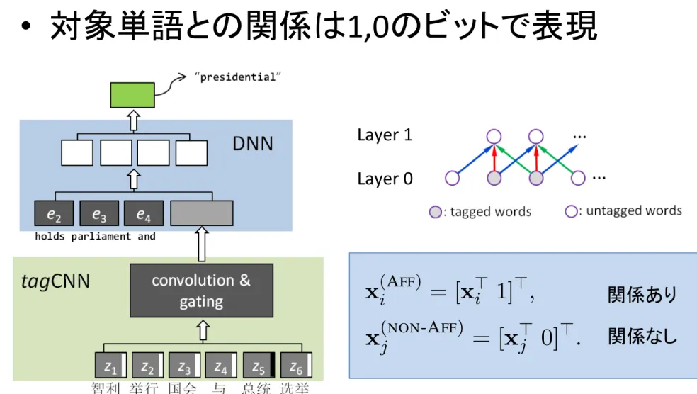
3.2 tagCNN
tagCNN inherits the convolution and gating
from generic CNN (as described in Section
3.1), with the only modification in the input
layer. As shown in Figure 2 (b), in tagCNN,
we append an extra tagging bit (0 or 1) to the
embedding of words in the input layer to
indi-cate whether it is one of affiliated words
x
(Ai FF)= [x
>i
1]
>, x
(NON-AFF)
j
= [x
>j0]
>.
Those extended word embedding will then be
treated as regular word-embedding in the
con-volutional neural network. This particular
en-coding strategy can be extended to embed more
complicated dependency relation in source
lan-guage, as will be described in Section 5.4.
This particular “tag” will be activated in a
parameterized way during the training for
pre-dicting the target words. In other words, the
supervised signal from the words to predict
will find, through layers of back-propagation,
the importance of the tag bit in the “affiliated
words” in the source language, and learn to put
proper weight on it to make tagged words stand
out and adjust other parameters in tagCNN
accordingly for the optimal predictive
perfor-mance. In doing so, the joint model can
pin-point the parts of a source sentence that are
rel-evant to predicting a target word through the
already learned word alignment.
3.3 inCNN
Unlike tagCNN, which directly tells the
loca-tion of affiliated words to the CNN encoder,
in
CNN sends the information about the
pro-ceeding words in target side to the
convolu-tional encoder to help retrieve the information
relevant for predicting the next word. This is
essentially a particular case of attention model,
analogous to the automatic alignment
mecha-nism in (Bahdanau et al., 2014), where the
at-23
あるノードからの入力