テクスチャ解析による夜間海面波浪状態の
ニューラルネットワーク学習
森元映治
1 †・中村誠
1Texture Analysis for Training of a Neural Network in
Identification of Ocean Surface Wave Conditions at Night
Eiji Morimoto 1 † and Makoto Nakamura 1
Abstract : A system for automatic monitoring of wave conditions in littoral waters was constructed. Based on previously reported findings using daytime ocean surface images, the ability of the system to use nighttime images was investigated. Texture analysis of ocean surface images was performed on infrared images, and the characteristic quantities of these results were compared with wind force. Two analytical methods were used to extract the image characteristics of the quantitative result: the spatial gray-level dependence method and the gray-level difference method. A multilayer neural network was trained to predict ocean wind velocity by error back-propagation. The specified conditions and optimal ocean surface images were then compared to the network structure and learning conditions to evaluate the effectiveness of this system and to assess its limitations.
Key words : measurement, sea surface, texture, neural networks, winds
1 Department of Ocean Mechanical Engineering, National Fisheries University †Corresponding author : [email protected]
Introduction
For members of the fishing industry, as well as ship operators and marine safety authorities, a knowledge of ocean wave conditions is very important. Ocean surface conditions have an inestimable impact on the efficiency and safety of fishing and maritime activities in the coastal waters of Japan; such activities extend from the automated navigation of trawlers to the more mechanical tasks of fishing, as well as the installation, maintenance and management of moored floating equipment, aquaculture rafts and fixed nets. This study attempted to develop a system that automatically detects ocean wave conditions using images of the ocean surface. A previous report addressed surface conditions during the day1). However, in this study,
infrared nighttime images were used to facilitate the measurement and monitoring of ocean wave conditions for a full 24-hour period. The wave conditions were subjected to texture analysis and digitized, and these data were then used to train a neural network that could be applied to recognizing and predicting wave conditions.
Texture Analysis
“Texture” refers to the large- and small-scale patterns in an image. As such, texture is not restricted to being a characteristic of highly ordered artificial objects, such as rows of blocks etc., rather, it can also be used to characterize natural phenomena, such as trees or the surface of water. Thus, monochromatic
surfaces can have textures with no variation in color density.
These structural and statistical analyses of texture can be used to derive the characteristic quantities of the texture in the image2),3). In texture analysis at the structural level, the basic elements constituting straight lines, points and other textural components are extracted from the image and characteristic quantities are revealed using rules that describe their spatial relationships. In this way, the constituent elements of the target image can readily be distinguished from artificial textures. In texture analysis at the statistical level, the color density of each pixel is examined for uniformity, directionality, variations in contrast, and other characteristic quantities. Since structural regularities, with respect to points and lines, were not observed in the data captured at the ocean surface in this study, the statistical level of texture analysis was considered appropriate for the current case.
Spatial gray level dependence method
Figure 1 shows the frequency at which the color densities (gray levels) of a pair of pixels (x1,y1) and (x2,y2) in a specified spatial relationship (d,θ) match with a density pair f(x1,y1)=i, f(x2,y2)=j. The probability of this match is defined by Sθ(i,j).
θ, which is the angle between a line joining the pixel pair and a horizontal line, can take the four values of 0º, 45º, 90º and 135º. The distance between the pixel pair under consideration is d in the θ direction. The procedure for creating the gray level cooccurrence matrix P(i, j│d,θ) is as follows. A pair of pixels is
selected as the density pair when a second point lies at distance d in the θ direction from the first point. Next,
the color density values of the pair are determined; if these densities are i, j, then the terms are summed to correspond to the terms of P(i, j│d,θ). Either of the
two members of the pair is allowed to have either gray level. The gray level cooccurrence matrix then has the size N × N, where N is the number of gray levels in the image.
The values of the characteristic quantities found by texture analysis can be determined using the following equations. Energy; ・・・・・・(1) Entropy; ・・・(2) Correlation; ・・(3) Local infirmity; ・・・・・・・(4) Momentum; ・・・・・(5) where,
i, j: Pixel color density
Sθ: Probability that a pixel at distance in the direction from a pixel of density in the image will have density
θ: Angle with respect to the horizontal by a straight
line between two pixels
d: Distance from a pixel of density to a pixel of
density
vx,vy: Mean color densities σx,σy: Variance of color density
Gray level difference method
We find the probability f(i,δ) that the difference i in the densities of two points separated by a constant displacement δ = (d,θ) (see Figure 1), and use this probability to calculate the characteristic quantities. The characteristic quantities identified by texture analysis can be identified using the following equations:
Contrast;
・・・・・・(6)
Angular second moment;
・・・・・・(7)
Entropy;
・・・・(8) Mean;
・・・・・・・(9)
Inverse differential moment;
・・・・・・(10)
where
N: Color density of pixel
i: Difference between density value L at (x1, j1) and
density value M at (x2, j2)
f: Probability that the color density difference will be i
Neural Network
An “artificial neural network” refers to mimicking the data processing that occurs in the cells (neurons) of the human brain using a computer. Numerical models perform the role of neurons, and the data-processing structure consists of a network of interconnected models4). This process facilitates numerical modelling of a system based directly on sets of input and output data, without equations. Figure 2 shows a model of a neuron.
x1,x2,x3...,xn in the figure correspond to the inputs,
w1,w2,w3...,wn correspond to the combination loads of
the paths, and y represents the output. If xi (i=1,2,3...n)
represents the input signal from the ith neuron, w
i
(i=1,2,3...n)represents the combination load, S is the sum of input signals from all other neurons, and fh is
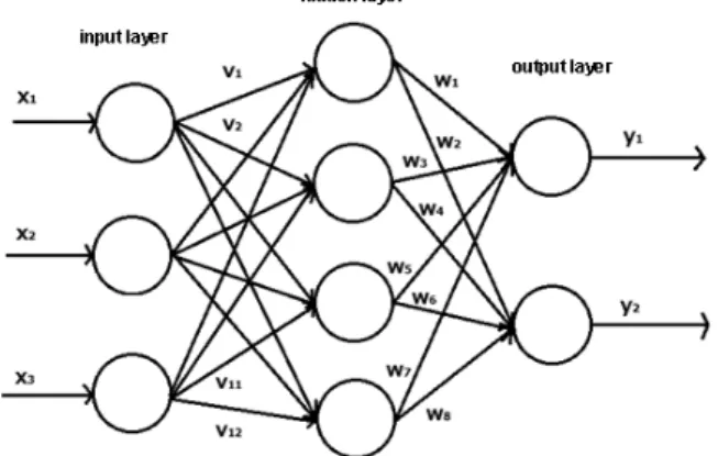
the sigmoid function, then we can obtain the following expression: ・・・・・(11) Output y is, ・・・・(12) A multilayer neural network shown in Figure 3 consists of an input layer, an intermediate layer and an output layer. There are no interconnections
within a layer in this type of neural network; a signal proceeds in a single direction, from the input layer through the intermediate layer to the output layer. This characteristic enables the network to learn faster than an interacting neural network.
Experiments and Results Textural analysis of wave images
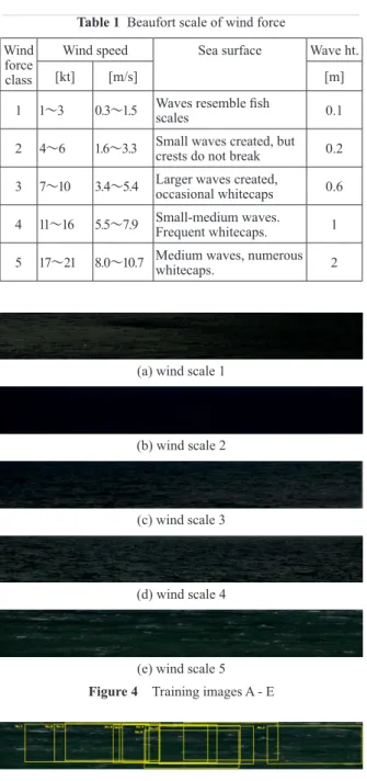
The Beaufort wind scale5) shown in Table 1 was used as an indicator of the wave conditions shown in the different images. Figures 4 provide images of training patterns.
Using image analysis software, the training images were analyzed using both the spatial gray level dependence method and the gray level difference method. Portions samples of the images were employed, as shown in Figure 5. The sample size was 500 × 200 (width x height) pixels.
id
Figure 2 Numerical model of neuron
Learning was performed using a neural network. The values for the characteristics of extracted energy, entropy, correlation, local uniformity and inertia were calculated. The color indices were classified as red, green or blue during analysis, but these were limited to just one color for comparison in Figure 6. No particularly prominent characteristics were found in this analysis, so red was employed as an index for the remainder of the experiment.
A network with inputs that consisted of energy, entropy, correlation, local uniformity and inertia, and an output of wind scale was created. Once the neural network had been trained, the prediction was calculated as output. The learning conditions were set for the neural network, which was trained to assess the relation between the wave image and wind scale. Table 2 shows the parameters for learning conditions.
Texture analysis of unclassified images
An analysis of images with unknown wave conditions was performed using the same procedure as described for the training data. Figures 7 show wave images F, G and H for which the wind scale was unknown.
(a) wind scale 1
(b) wind scale 2
(c) wind scale 3
(d) wind scale 4
(e) wind scale 5
Figure 5 Training image E marked to show cut-out portion Figure 4 Training images A - E
Figure 6 Local uniformity of colors
Table 2 Learning conditions used for the neural network
Learning iterations 10000 Permissible error 0.1 Number of hidden units 10 Random numbers 1 Fraction 100.% Lower limit -1 Upper limit 1 (a) Image F (b) Image F (c) Image H
Figure 7 Unclassified images Table 1 Beaufort scale of wind force
Wind force class
Wind speed Sea surface Wave ht. [kt] [m/s] [m] 1 1~3 0.3~1.5 Waves resemble fish scales 0.1 2 4~6 1.6~3.3 Small waves created, but crests do not break 0.2 3 7~10 3.4~5.4 Larger waves created, occasional whitecaps 0.6 4 11~16 5.5~7.9 Small-medium waves. Frequent whitecaps. 1 5 17~21 8.0~10.7 Medium waves, numerous whitecaps. 2
Learning with neural network and predicting winds The analytical results from the training images were used for training. Figure 8 shows the predicted wave conditions based on the teaching and unclassified images. There are some concerns about the numerical stability of the predictions inferred from images A – C, but the scatter was low in the unclassified image F, and the values were relatively stable.
Predictions with gray level difference method The neural network was trained using the data obtained with the spatial gray level dependence method. The contrast, angular second moment, entropy, mean, and inverse difference moment obtained with the gray level difference method were used for training using the same procedure described above. Figure 9 shows the results.
In this study, the gray level difference method was found to be less suitable for training than the spatial gray level dependence method. Still, since the greater the wind scale, the greater the precision achieved by the gray level difference method, the gray level difference method may well be effective for predicting wave conditions under high winds, despite the lack of
robust findings observed in this study.
Predictions for analytical regions of varying sizes Instead of using an image measuring 500 × 200 pixels, we increased the size of the image to 1000 × 200 pixels, and show the results in Figure 10. The results showed that the findings obtained from the analysis were stable when the size of the image area was doubled. Interesting, more precise predictions were obtained for cases A – C, whose values had not been very stable when images measuring 500 × 200 pixels were measured.
Predictions obtained from unclassified images after changing analytical region size
Figure 11 shows the predictions of the trained network obtained from unclassified images F, G and H. Although the results shown in image G were not considered very stable, the values obtained from image H were stable. When these findings were compared with the Beaufort wind scale, image G was classified as wind scale 3, and image H, as wind scale 2, essentially
Figure 8 Wind scales of training images and prediction results
from teaching and unclassified images
Figure 9 Predicted results using the gray level difference method
Figure 10 Predicted results obtained using a 1000×200 pixel
image method
Figure 11 Prediction results using 1000×200 unclassified
matching the predicted results.
Effect of changing the number of units in the intermediate layer
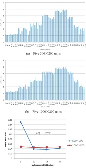
The number of units comprising the intermediate layer of the three-layer neural network was increased from 5 to 15 and then to 20 units, and the obtained results were compared in Figure 12.
Figure 12(c) shows the error between the predicted values and the estimates based on visual observations when the number of units in the intermediate layer was changed from 500×200 to 1000×200. When the number of units in the intermediate layer was 5 units and the image was 500×200 pixels, convergence
was 75% at 10,000 learning cycles, so learning was forcibly terminated at this cycle number. No notable changes were observed in the results obtained using an intermediate layer with other sizes.
Summary
Although this experiment employed nighttime images of ocean surface waves, which provide comparatively little detail of the photographed. Two analytical methods were used here, spatial gray level dependence and gray level difference; within the present range, the spatial gray level dependence method showed superior predictivity. The gray level difference method did not provide satisfactory results in the present study. This is probably because of the difficulties associated with extracting characteristics using that method and nighttime images, which typically have characteristic quantities that are relatively poorly defined. However, the accuracy of the gray level difference method did improve as the wind scale increased. It is therefore possible that that method could be used, with appropriate pre-processing, to improve prediction accuracy.
Some improvement in accuracy was observed under calm conditions when the size of the analytical region was increased. This improvement was attributed to obtaining more accurate values for the characteristic quantities from larger extracted portions. However, when the wind conditions were strong, the accuracy deteriorated as convergence increased.
Provided that convergence was obtained in this experiment, the number of units in the intermediate layer did not have any particular affect on accuracy. Although color did not markedly affect analytical results, larger extracted images could be beneficial, as images with 1000×200 pixels provided more accurate data than images measuring 500×200 pixels, at lower wind scales.
The following are recommended topics for future research: The efficacy of both analytical methods used in this study should be reviewed at higher wind scales; the minimum practicable size for an image to provide accurate predictions should also be identified.
(a) Five 500×200 units
(b) Five 1000×200 units
(c) Error
References
1) Morimoto E, Nakamura M : Neural Network Learning of Ocean Wave Condition by Texture Analysis, J Nat Fish Univ, 60, 173-181 (2012) 2) Takagi M, Shimoda H : Handbook of Image
Analysis. University of Tokyo Press, Tokyo (1991)
3) Murakami S : Image processing Engineering. Tokyo Denki University Press, Tokyo (1996) 4) Looney G : Pattern Recognition Using Neural
Networks. Oxford University Press, (2004) 5) Isozuka I : ABC for Wave Analysis.