位相不変量を用いたDNA結び目に対する応用解析 (生命現象と関連した非線形問題の数理)

Applied

analysis

to DNA knot

by topological

invariants

位相不変量を用いた

DNA

結び目に対する応用解析

Takashi Yoshino and Isamu

Onishi

(Hiroshima University)

吉野 貴史、大西 勇 (広島大学 大学院理学研究科 数理分子生命理学専攻)

Contents

12

1.1 2 1.2 2 1.3 3 1.4 4 1.5 4 1.6 6

2 PreparationsfromTopology 7

3 Simulations 8

3.1 Alexander polynomial

. . .

.

. . .

.

. . . .

.

.

.

. . . .

8

3.2 Jones polynomial .

.

. . .

.

. . .

.

. .

.

. . .

. .

. .

.

. . . .

.

. .

. . .

. . . .

. .

.

.

10

4 Results and Disucussion 11

4.1 Comparisonofthe results byAlexander polynomial and those by Jones polynomial.

. . .

11

4.2 Comparison of the results of thesimulation and those ofbiological experiments . . .

. .

. 12

1

Introduction

1.1

Topological

Structures

of

a

DNA

The structure of DNA isa double helix, much like

a

ladder that is twisted into

a

spiral shape. In 1953

the double-helix structure of

a

DNA

was

proposed by J. D. Watson and F. H. Crick with technique

to build

a

molecular model. The double helix is the ideal model that J. D. Watson and F. H. Crick

arrived at from many studies about a DNA and

seven

next importantcharacteristics are emphasized in

the structure.

1. The double helix is formed by two polynucleotide.

2. A purine and apyrimidine ringorient it in the inside of the double helix.

3. The base in complementary relations is bound by hydrogen bond.

4. There is 10.4 base pair per spiral 1 round per minute.

5. As for two polynucleotide ofthe double helix,

a

direction is

reverse

(reverse parallel) each

.

6. Double helix has two kinds ofgrooves, the majorgroove and the minor groove.

7. The doublehelix is clockwise twining (right handed).

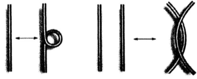
Whenadouble-stranded DNA of the double-helix structureis twisted

more

orit is untied, the double

helix is

more

twisted

as

a whole. These

are

called the supercoiled structure (a positively supercoiled

DNA is the former and

a

negatively supercoiledDNA is the latter, respectively).

The ringed supercoiled DNA closed by covalent bond has “the twist” and “the writhe”. “The twist“

is the spiral number of revolutions that

one

chain surrounds the chain ofthe other, that is the number

oftimes that

one

chain completely coils the chain of the other. “The twist$\rangle$

in a right-handed spiral is

defined as plus. “The writhe” is

a

number that the double strand coils oneself or the double strand is

coiled cylindricallylikethecordof the telephone. The total valueof”thetwist” and“

the writhe” cannot

be changed unless we cut off the DNA. As

an

enzyme changing topological structure of the DNA, we

takethe transpososome and the topoisomerase for

an

example.

1.2

Transpososome

The transpososome is a complex of the transposon and the transposase. The transposon is the base

sequence which

can

perform

a

transposition on the genome in a cell. An enzyme called transposase,

which transposononeselfencodes, is necessary for transposon DNA to perform transposition.

The transposon has the reverse repetitive sequences on the end and the transposase recognizes this

arrangementand cutsa transposonfrom a DNA arrangement. Therefore it is necessary for transposase

to cut each DNA chain at each end of the transposon. The cutting happens in a linkup with the host

DNA adjacent to atransposon. The transposase cuts the DNAto leave the reverserepetitivesequences

(or the part) in the place where atransposon originally

was

in. After a transposon

was

cut, the end of

thetransposon DNA that is the end that transposasecut firstattacks the DNA phosphodiester bond ofa

newinsertionpart. ThisDNA domainiscalledthe target DNA. Because thetranspososome

was

formed,

twoends ofthe transposon DNA attack two chains ofthe same target DNA. As aresult ofattack, the

transposonDNA is bound by the covalent bond to the DNA of the target part.

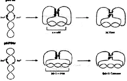
Although thetranspososomechanges topologicalstructuresof the DNA, differentproductsisexpressed

by theglobalstructure of theDNA [1]. Inthe twoplasmidsubstrates pSPIn and pSPDir, the loxP sites

(the targets for the Cre protein) are in inverted (head to head) and direct (head to tail) orientations,

respectively (Fig.1). _{Theydivideeach}plasmid _{into two domains shown in red and blue. Recombination}

mediated by the Cre tetramer would yield a DNA inversion product with pSPIn and apair of deletion

circles withpSPDir.

In a general case, if $n$ interdomainal supercoil nodes ($n$ being odd) were trapped in the unknown

that

an

odd number of trapped nodes would arrange the loxP sites of pSPIn in antiparallel alignment.

For the Cre deletion reaction in pSPDir,

an

additional node $(|n|+1=even)$ has to be introduced for

the antiparallel arrangement of the loxP sites (Lower

_area

_{ofFig.1). Theproducts}ofdeletionwould be

a

pair of catenated circles linked by $(|n|+1)$ crossings. Thege _{nodes arepreserved in the recombination}

products, and report on the DNA topology within the synapse. The location of the loxP sites in these

plasmids is such that the hybrid synapse has very little chance of accidentally acquiring interdomainal

nodes, depending

on

the loxP orientation.

$p\nu u$

$\alpha m$

$-r-$

Fig. 1 Cre Recombination from a Preassembled Synapse

1.3

Topoisomerase

The topoisomerase is theenzymewhich

can

change structures of the DNA by cuttingthesingle strand

or the double strand of the DNA temporarily.

Thetopoisomerase hastwotypes. TypeItopoisomerasescut thesinglestrand of the DNAtemporarily

and connect it again after dipping theother single strand. Type II topoisomerasescut the double strand

temporarily and close afterdipping another double strand which is not cut.

Bothaprokaryote andorganism withanucleus havetypeI andII topoisomerase whichcan

remove

the

supercoiledstructure fromthe DNA. Prokaryotes possess twostructurallysimilar type II topoisomerases,

Gyrase and Topo IV, which differ in their function. Gyrase generates negative supercoils, but Topo IV

relaxes positive supercoils. In addition, it has reported that Gyrase is strongly bound with DNA, but

Topo IV is weak [2].

The globalstructure ofDNAstrongly ties tothe expression pattem of DNA bythe propertyofTopo

IV and Gyrase, since the different DNA structure tends to produce different DNA modification even

under the

same

local condition. For example, when Gyrase

was

added to the positively supercoiled

DNA, Gyrase unties DNA since Gyrase generates

a

negatively supercoils, but when Gyrase

was

added

to thenegatively supercoiled DNA, Gyrase twists DNA more. Thus, the global structure ofthe DNA is

important foran enzyme.

It is known that the global topologicalstructures ofDNA tend to affect theexpression oftranscripts.

DNA is affected by other nucleic acids and enzymes in the process of DNA transcription. The global

structure of DNAstrongly ties tothe expression patternof DNA, sincethe different DNAstructuretends

to produce different DNA modification even under the same local condition. Then it has been reported

that the global topologicalstructures of DNA influences expression of transcripts by performing various

DNA in

a

phage.

1.4

Structures

of a

phage

A phage is

a

virus which infects bacteria. It is well known that It is well known that it has tails and

a

regular icosahedral head(see Fig.2). A phage is the simplest system to study

a

basic process of life.

The genomeis small generally and thegenomereproduceonly after invadingahostcell (abacteriacell).

Then

a

gene isexpressed. A genome tends to be rearranged while infection.

Because the system is simple,

a

phage

was

used verywell at the molecular biological dawn. Actually,

a

phagewas indispensable forthedevelopmentof this field. Thesystem is also most suitable for astudyof

theDNA replication, thegeneexpressionandbasic structuresof the recombination today. Furthermore,

a phage is important

as

a vector of the DNA recombination, and it is used to examine the activity

inducting variation ofvarious compounds.

Phages usually pack genomes (generally, DNA) to a mantle consisting of subunits of the protein. A

subunithas a one making headstructure (packing genomes) anda onemaking tail structure. The phage

particle is glued to the outside of the bacteria host cell with

a

tail and injects

a

phage genome to

a

cell.

Because each phage glues to

a

specific molecule (usually, protein) in the cell surface, only

a

cell having

a coping acceptor is infectedwith aphage.

A phage has a double-stranded DNA controlling

a

genetic informationin the head. The linearDNA

packed in the head ofphages forms various types of knots. As the part ofknots, Fig.3 shows knots $0_{1}$,

$3_{1},4_{1},5_{1},5_{2},6_{1},6_{2},6_{3},7_{1},7_{2},7_{3},7_{4},7_{5},7_{6}$ and $7_{7}$.

It is the important step of the DNA studies to investigate thefractions of various types of knots and

clarify the

reasons

of thephenomena.

Fig. 2 A bacteriophage

1.5

Results of biological experiments

$o_{\dagger \mathcal{O}^{3_{1}}\ ^{4_{1}}\mathfrak{H}^{5_{t}}\Phi^{5_{2}}\mathfrak{H}}$

$6_{1}$

馨

$6_{3}7_{l}\otimes\otimes^{\gamma_{l}}\oplus$ $7_{3}7_{4}\otimes\otimes^{\gamma_{s}}\otimes 7_{6}\^{7_{7}}\Re$

Fig. 3 Theprimeknotshavingbelow 7crossing

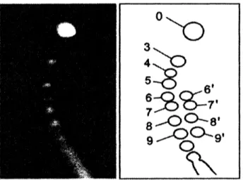
The DNA insidethe phage was examined types of knots which is made inside the phage and the

proba-bility by J. Arsuaga ct. al. [3]. First, purifiedDNAwasanalyzed by two-dimensionalgelelectrophoresis.

By gel electrophoresis, we can distinguish

some

knot types with the number of the

same

crossing

num-ber. To the direction of I of Fig.4, DNA samples

were

run

at 0.8$V/cm$ for 40$h$ at

room

temperature.

Aftera 90’ rotation ofthe gel, the direction ofIIofFig.4was

run

inthe same elcctrophoresis buffer at

3.4$V/cm$_for $4h$at room temperature. This gel electrophoresis segregated the linearDNA molecules and

segregated knots with six and more crossings to two groups. Knot populations of low crossing number

$\underline{1i}$

Fig. 4 Theresult of gelelectrophoresis by J. Ar- Fig. 5 The enlarged pictureof Knotpopulations

suagaet. al. [3] of lowcrossing number in Fig.4

Next, the projection obtained by this experiment

was

compared with the projection of known knot

typesto examine the knots corresponding DNA knots separated by electrophoresis (see Fig.6). The gel

velocityat lowvoltageof individual knotpopulationsresolved bytwodimensionalelectrophoresis (Right

ofFig.6) iscomparedwith the gel velocityat low voltage of twistknots $(3_{1},4_{1},5_{2},6_{1}$ and $7_{2})$ ofa $10-kb$

nicked plasmid (Center ofFig.6) and with known relative migration distances of

some

knot types (Left

ofFig.6). By thiscomparison,

some

knot typesof each population are distinguished, Inaddition to the

unambiguous knots $3_{1}$ and $4_{1}$, the knot population of five crossings matched the migration ofthe knot

$5_{1}$

.

The knot $5_{2}$ appeared to be negligible or absent. The knot population of

seven

crossings matched

the migration of the torusknot $7_{1}$ rather than the twist knot $7_{2}$. Yet, we cannot identify this gel band

as

the knot $7_{1}$, becauseother possible knot types of

seven

crossings cannot be excluded.

Then, several indicators led us to believe that the second arch ofthe gel ($6’\sim 9’$ ofFig.5) consists of

mainly compositeknots (seeDef.2.6 in Chapter 2). First,the archstarts at knot populationscontaining

six crossings, and

no

composite knots of fewer than six crossings exist. Second, the population of six

crossingsmatched themigrationat lowvoltage of thegrannyknot (compositeof

a

$3_{1}$ plus

a

$3_{1}$, indicated

as

$3_{1}\# 3_{1})$ , although the squareknot (theotherpossible compositeof six crossings, $3_{1}\neq-3_{1}$) cannot be

excluded. Third,consistent with the low amount of$4_{1}$ knots,the size of theseven-crossing subpopulation

isalso reduced; thus,anycompositeseven-crossing knotis$3_{1}\# 4_{1}(or-3_{1}\neq 4_{1})$. Theincreasedgel velocity

at high voltageof composite knots relative to prime knots (seeDef.2.5 in Chapter2) ofthe

same

crossing

$3_{1}$ $4_{1}$ $S_{7}$ 迦 $s_{1}us_{\uparrow\ovalbox{\tt\small REJECT} 6_{1}}$ $7_{1}$ $7_{2}$

Fig. 6 Upper areaof the gel picture showing knot populations of low crossing number

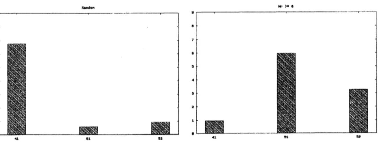
Densitometer readings confirmed theapparent scarcity of the knot of four crossings (knot $4_{1}$) relative

to the other knot populations in the main arch of the gel. Fig.7 shows the results of the fractions of

knots $3_{1},4_{1},5_{1}$ and $5_{2}$ by biological experiments. However, the scarcity of the knot $4_{1}$ relative to the

knotof three crossings (knot $3_{1}$) and to other knotpopulationsis enhanced if

we

make the correction for

DNA molecules plausibly knotted outside the viral capsid. In such a case, one can predict that 38% of

the total number of observed $3_{1}$ knots and 75% of the observed$4_{1}$ knots are formed by random knotting

in free solution.

Fig. 7 The results of thefractionsofknots$3_{1},4_{1},5_{1}$ and$5_{2}$ by biologicalexperiments [3]

1.6

Outline of this

study

Tostudy the geometryofthe DNA inside the phage, we simulated thefractions ofthe varioustypesof

knots and compared to those ofbiological experiments.

First,

we

simulated under the assumption that DNA knotsinside the phage

were

generated at random.

WithMersenne Twisterwe randomly made the knot topology having$n$ crossings $(n=3,4, \cdots, 8)$

.

This

process

was

repeated 1,000,000 times to obtain 1,000, 000 knots. Then we classified these knots with

and

we

considered the

mean

value of all trials as the conclusive fractions of the above-mentioned types of knots.

Next,

we

examined “the writhe value” $Wr$ at each crossing. After eliminating matrices having the

small value of the total amount $\sum Wr$,

we

performed the

same

simulation

on

the remaining matrices.

The fractions of the knots $3_{1},4_{1},5_{1}$ and $5_{2}$ after considering “the writhe value”

were

similar to the

biological results.

2

Preparations

from

Topology

Def. 2.1 (Alexander matrix) Let $G$ be a group and let $\alpha$ : $Garrow G/[G, G]$ be the Abel map. The

image $A(G, \alpha)$ of Jacobian by the Abel map $\alpha$ is called Alexander matrix of$G$

.

Def. 2.2 (Alexander polynomial) The$g$. $c$. $d$. of determinant of

$(n-1)x(n-1)$

submatrix of$n\cross n$

Alexander matrix is called Alexander polynomial.

Def. 2.3 (Trivial knot) Let $K\subset S^{3}$ be

a

knot. If there exists $K\subset S^{2}$ for

a

two-dimensional sphere

$S^{2}\subset S^{3}$, then _$K$ is calledthe trivial knot,

Def. 2.4 (Connected

sum

ofknot) Let $K_{1}\subset S^{3},$ $K_{2}\subset S^{3}$ be knots and let $B_{1}=S^{3}-intN(x_{1})$,

$B_{2}=S^{3}-intN(x_{2})$ for points $x_{1}\in K_{1},$ $x_{2}\in K_{2}$

.

If

we

set $Si=\partial B_{i}$ $(i=1,2)$, then $S_{i}$ is

a

two-dimensionalsphere and $K_{i}\cap Si$ is

a

one-dimensional sphere in $S_{i}$.

Then

we

identify$S_{1}$ with $S_{2}$ and identify$K_{1}\cap S_{1}$ with $K_{2}\cap S_{2}$ by ahomeomorphic mapping $(S_{1},$ $K_{1}\cap$

$S_{1})arrow(S_{2}, K_{2}\cap S_{2})$, and

we

connect $(B_{1}, K_{1}\cap B_{1})$ and $(B_{2}, K_{2}\cap B_{2})$

.

The obtained knot $K\subset S^{3}$ iscalled the connected sumof$K_{1}$ and $K_{2}$, we use the notation$K_{1}\# K_{2}$

.

Conversely, it is called that $K$ is decomposed $K_{1}$ and $K_{2}$

.

Def. 2.5 (Prime knot) For thearbitrary decomposition $K=K_{1}\# K_{2}$ of the knot$K$, if at least

one

of

$K_{1}$

or

$K_{2}$ is the trivialknot, then $K$ is called the prime knot. However, we define that the trivial knot

is not the prime knot.

Def. 2.6 (Composite knot) If there exists a decomposition $K=K_{1}\# K_{2}$ of the knot $K$ such that $K_{1}$

and$K_{2}$ is the non-trivial knotwhich is not prime, then $K$ is called the composite knot.

Def. 2.7 (Skein relation) Let$t$bethenonzerocomplexnumberand let $L_{+},$ $L$-and$L_{0}$be three knots

thatonly one part crosseslike a Fig.8 and the other part is totally same.

Then

$tV_{L_{+}}(t)-t^{-1}V_{L_{-}}(t)=-(t^{1/2}-t^{-1/2})V_{L_{0}}(t)$

is called Skein relation.

$\backslash \nearrow\backslash L_{+}$ $\backslash _{L_{\sim}}\nearrow’$ $)_{L_{O}}($

Fig. 8 Three knots $L+,$ $L$-and $L_{0}$

Def. 2.8 (Jones polynomial) The polynomial $V_{L}(t)$ such that Skein relation hold is called Jones

Def. 2.9 (Bracket polynomial) The polynomial $<D>$ ofone variable $A$ obtained by applyingnext

three rules tothe link diagram $D$ is called Bracket polynomial:

(i)

$<U>=1$

;

(ii) $<DU>=-(\mathcal{A}^{2}+A^{-2})<D>$; (iii) $<’\backslash ’>=A<\wedge>+A^{-1}<)$$(>$_;

$<^{\backslash }\Gamma\backslash >=A<)(>+A^{-1}<\wedge>;\vee$

where $U$is$a$ trivialknot, $DU$is anunion with

a

trivial knot and weapply (iii) locally at each crossing

ofthe link diagram.

Then for the link diagram $D$ of

an

arbitrary knot $L$ withthe direction, Jones polynomial $V_{L}(t)$ has a

relation with Bracket polynomial $<D>$ by

$V_{L}(A^{-4})=(-\mathcal{A}^{3})^{-\omega(D)}<D>$,

where$\omega(D)$ is thesum of”thewrithevalue” ateach crossingofthe link diagram$D$ (seeSection 3.1.1),

It is known that the Alexander polynomial and Jones polynomial, which are the invariant forknots,

is effectively used for the classification of knots based on the topology. We can classify all prime knots

having below 8 crossing by a combination of the value of $\Delta(-2)$ and $\Delta(-3)$ when we

use

Alexander

polynomial $\Delta(t)$

.

Then we can distinguish the mirror images of knots and knots having

more

crossings

when

we

use

Jones polynomial.

3

Simulations

3.1 Alexander

polynomial

3.11 Elementsof Alexander matrix

Weshall project the knot

on a

placealonganarbitrarily chosenaxis,while drawingbreaks at the crossing

points in the part of the

curve

that lies below. Now theprojection of the knot amounts to the set of

segmentsofcurves, which are called the generators. Let us fix arbitrarily the direction ofpassageofthe

generators and number them, havingselectedarbitrarily thefirst generator. Thecrossing that separates

the kth and $(k+1)$th generators will be called the kth crossing. The crossings are of two types (see

Fig.9). The writhe value $Wr$ _is $Wr=-1$ at type I crossing and $Wr=1$ _{at type II crossing. The}

elements ofAlexander matrix$A(t)$ are defined asfollows [4].

1. When $i=k$

or

$i=k+1$, independently of the type of crossing: $a_{kk}=-1,$ $a_{kk+i}=1$

.

2. When $i\neq k,$ $i\neq k+1$, for a type Icrossing: $a_{kk}=1,$ $a_{kk+1}=-t,$ $a_{ki}=t-1$.

for

a

type II crossing: $a_{kk}=-t,$ $a_{kk+1}=1,$ $a_{ki}=t-1$.

3. All the elementsexcept $a_{kk},$ $a_{kk+}1$ and $a_{ki}$ are zero.

Here $k$ is the number of crossing and $i$ is the number of the overpassinggenerator. Then these

$-\ovalbox{\tt\small REJECT}-$ $-\ovalbox{\tt\small REJECT}-$

Fig. 9 The type I crossing (left) and the typeII crossing (right)

3.1.2 Generation of Alexander matrix

First,

we

fix the dimension $n$ of the Alexander matrix from 3$\sim$8 with Mersenne Twister at random.

Second,

we

fix the element $a_{kk}$ $(k=1,2, –, n)$ of $n\cross n$ matrix $\mathcal{A}(-2),$$A(-3)$ $(n=3,4, \cdots, 8)$

substituted $t=-2,$$t=-3$ with Mersenne Twister

as

to satisfy above list. When $i\neq k$ and $i\neq k+1$,

we

take$i$ with Mersenne Twister at random ($i$ must not take $k$ and $k+1$). This work is repeated from

$k=1$ to $k=n$ andwemake the $n\cross n$ matrixcorresponding to the random knot.

3.1,3 _{Reidemeister moves}

ByReidemeister moves, we untie thepartwhich

can

untie of the knot. Reidemeister

moves

I,II (Fig.10)

arethe next operation $[$4$]$.

I. Ifthe kth row contains onlytwo

nonzero

elements $a_{kk}=-1$ and $a_{kk+1}=1$, then we should

add the column $k$ to the column $k+1$

.

Thenwe delete $tI_{1}e$ kthcolumn and the kth row and

renumber the

rows

and column afresh.

II. If in two adjacent rows ofthe matrix having the numbers $k$ and $k+1$ elements having the

value $t$–llie in

a

single column and elements equal to $t-1$

are

lacking in the $(k+1)th$

column, then we should add the kth column to the $(k+2)$th, and then delete the kth and

$(k+1)$th

rows

and columns and renumber all the rowsand columns afresh.

The above list I and IIcorrespond Reidemeister

moves

I andII, respectively.

Fig. 10 ReidemeistermovesI (left), II (right)

3.1.4 Classification of knots

Weestimate the value $\Delta(-2),$ $\Delta(-3)$ ofthe determinant of the $(n-1)\cross(n-1)$ submatrix and classify

knots by the combination of the value of the determinant. Here,

we

removed all rows and columns from

the first row and column to the nth row and column one by one. Then we treated

as

a knot when

integer).

3.1.5

Reliability ofthesimulation

Wegave1, 000,

000

matrices at random and counted the numberwhichgeneratedeach knotand estimated

the fractions. These trials

were

repeated 100 times and we considered the

mean

value of all trials

as

the

conclusive fractions of the types of knots.

3.1.6 Addition of “the writhe”

After the simulation of the random matrices, we employed “the writhe value” in the simulation. we

examined “

the writhe value $Wr^{:}$ at each crossing. After eliminating matrices havingthe _small value of

the totalamount $\sum Wr$,

we

performed the

same

simulation

on

the remaining matrices.

3.2 Jones

polynomial

3.2.1

Recurrent algorithm of Bracket polynomial

Because we can find Jones polynomial from Bracket polynomial ifwe find “the writhe value” ofthe

knot, weconstitute algorithm by Bracket polynomial [5].

For

an

arbitrary link diagram $D$,

we

paint with two colors of the black and white

so

that adjacent

domainsdo not become thesame color. Here, infinitedomain is the white. Next, wechoose onepoint in

each black domain. If two black domains

are

adjacent,

we

link the point that

we

chose ofeach domain

andwe establish thesignof theedgebasedon Fig.11. Thus, the plane graph$S$with thesign is obtained.

$+$ –

Fig. 11 The sign intwo adjacent black domains

We definethat $S\backslash e$is the graphwhichdeleted the edge$e$fromthegraph $S$ and $S/e$is thegraphwhich

contracted the edge $e$ from $S$ (that is the edge $e$ is condensed andthe top ofboth ends correspond

one

point). Then we define that the loop is the edge where boih ends are the same tops and the bridge is

theedge where the connected component of thegraph increases

one

when the edge is deleted.

It is known that the contraction/deletion formula ofthe edge holds for graph $S$ with thesign. For

example, when the edge linking two adjacent black domains is positive, the operation which tie two

black domains and the operation which divide two black domains is equivalent to the contraction and

the deletion, respectively.

$<S>=A<S/e>+A^{-1}<S\backslash e>$

Then when the edge $e$ is the positive bridge, $S\backslash e$ is disconnectedness (that is the number of the

component of the knot corresponding to $S\backslash e$ increases one), but $S\backslash e$ and $S/e$ is the isomorphism, and

the following relations hold betweenthem.

$<S\backslash e>=(-A^{2}-A^{-2})<S/e>$

Therefore, they hold thefollowingrelations when the edge $e$ is thepositivebridge.

$<S>=A<S/e>+A^{-1}<S\backslash e>$ $=-\mathcal{A}^{-3}<S\backslash e>$

It is similar in the

case

of the negative bridge

or

theloop too, therefore they hold the following

recurrence

relations.

$<S>=\{\begin{array}{ll}-A^{-3}<S/e> if e is the positive bridge-A^{3}<S/e> if e is the negative bridge-A^{3}<S\backslash e> if e is the positive loop-A^{-3}<S\backslash e> if e is the negative loopA<S/e>+A^{-1}<S\backslash e> if e is positive (otherwise)A<S\backslash e>+A^{-1}<S/e> if e is negative (otherwise)\end{array}$

Thenwhen $S$ consists of

one

edge (thepositive bridge $C^{+}$, the negative bridge $C^{-}$, the positive loop

$L^{+}$, thenegative loop $L^{-}$), Bracket polynomials hold the following relations.

$<C^{+}>=-A^{-3},$ $<C^{-}>=-A^{3},$ $<L^{+}>=-A^{3},$ $<L^{-}>=-A^{-3}$

Furthermore, when the edge set of$S$ is the empty, Bracket polynomial has 1 from 2.9 (i).

3.2.2 Generation ofthe random plane graph with the sign

First, wefix the number of the topfrom 2$\sim$8 with Mersenne Twister at random and alsofix the number

ofthe edge from 3$\sim$8at random. Next, we choose tops linked each edges at random and give the sign

at random. Thus, we generate therandom plane graph with the sign.

3.2.3 Classification of knots

We substitute 2for variable $A$ of Bracket polynomial and evaluate the

recurrence

algorithm of Bracket

polynomial for the given graph. Thenwe classify knots by the value whichwas finally obtained. Here,

because we considered the difference of the value of “the writhe value” of the knot, we also treated as

the knot when the value whichwas finallyobtained was different $(-2)^{3m}$ times ($m$ is aninteger).

3.2.4

Reliability of the simulation

Wegave1, 000,000matrices at random and counted the number which generated each knot and estimated

the fractions. These trialswererepeated 100 timesand weconsideredthe

mean

valueof all trialsas the

conclusive fractions of thetypes ofknots.

4

Results and

Disucussion

4.1

Comparison of the results

by

Alexander polynomial and those by

Jones

polynomial

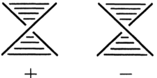
When knots

were

generated at random, Fig.12 shows the results by Alexander polynomial and Fig.13

shows thoseby Jonespolynomial ($*$inFig.13represents themirror imagesofknots). In bothresults, the

fraction of the knot$3_{1}$

was

the highest, the fractions of$4_{1}$

was

the second highest, $5_{2}$ was the third and

$5_{1}$

was

thefourth. In knotshaving6crossing, the fraction of the knot $6_{2}$

was

thehighest, the fractions of

63

was

the second and $6_{1}$

was

the third. Furthermore, by theresults by Jones polynomial, the fractions

Fig. 12 Fractions distinguished knots generated

at random byAlexanderpolynomial

Fig. 13 Fractions distinguished knotsgenerated

at random by Jones polynomial

4.2 Comparison

of

the results

of the simulation and

those

of biological

experiments

About knots $3_{1},4_{1},5_{1}$ and $5_{2}$,

we

compare the results of the simulation by Alexander polynomial with

theresults of biological experiments. The fraction of knot types that emerged in biologicalexperiments

conducted by J. Arsuaga et. al. [3] is shown in Fig.14. In the biological experiments the fraction of

the knot $3_{1}$

was

the highest and the fractions of $5_{1}$ was the second highest, while $4_{1}$ and $5_{2}$ were low

(Fig.14). In contrast, the fraction of knots that were computationallygenerated atrandom (Fig.15)

was

very different from theresults ofbiological experiments. InFig.15, the abundance of$4_{1}$

was

higherthan

$5_{1}$ and $5_{2}$

.

Fig. 14 Theresults ofbiological experiments by Fig. 15 Fractions oftheknots $3_{1},4_{1},5_{1}$ and$5_{2}$

J. Arsuagaet. al. [3] generated at random

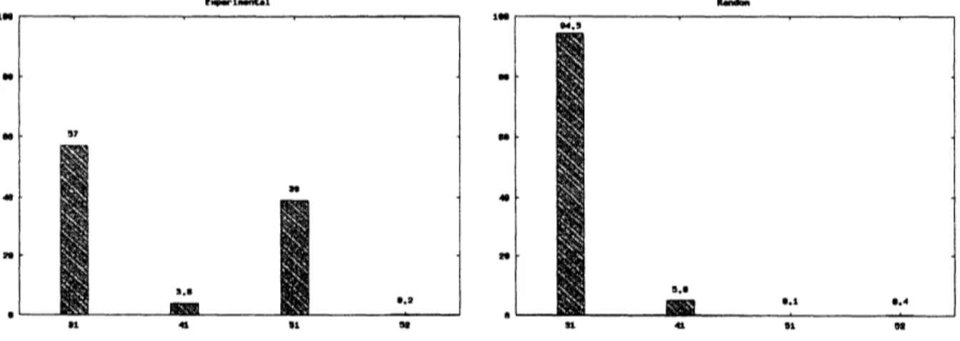
However, employing “the writhe value” in the simulation changed the results. The fractions of the

$w\rangle\cdot\cdot$

Fig. 16 Fractionsoftheknots$4_{1},5_{1}$ and$5_{2}$

gen-erated at random

4.3 Disucussion

and

Future problems

Fig. 17 Fractions oftheknots$4_{1},5_{1}$ and$5_{2}$ after

examining“_{the writhe value”}

We conclude that DNAknots inside the phage arenot generated at random andthey would have some

bias beingrelated to “_{the writhe value”.}

Infuture, wewill devise simulation methods fordistinguishing knots having

more

crossings.

References

[1] S. Pathania, M. Jayaram and R. M. Harshey, Path

_of

$DNA$ within the $Mu$ 7branspososome:

[Zlnans-posase Interactions Bridging Two $Mu$ Ends and the Enhancer Trap Five $DNA$ Supercoils, Cell,

Vol.109, (2002), 425-436.

[2] G. Charvin, T. R. Strick, D. Bensimon and V. Croquette, Topoisomerase IV Bends and

overtwtsts

$DN\mathcal{A}$ upon Binding, Biophysical Joumal, Vol.89, (2005), 384-392.

[3] J. Arsuaga, M. Vazquez, P. McGuirk, S. Trigueros, D. W. Sumners and J. Roca, $DNA$ _{knots reveal}

a chiral organization

_of

$DN\mathcal{A}$ inphage capsids, PNAS, Vol.102, (2005), 9165-9169.

[4] M. D. Frank-Kamenetskii and A. V. Vologodskii, Topological aspects

_of

the physics

_of

polymers: The

theory and its biophysical applications, SOV.Phys.-Usp.(Engl.Transl.), Vol.24, (1981), 679-696.

[5] K. Sekine, H. Imai and K. Imai, Computation

_of

the Jones Polynomial, Transactions of JSIAM,