Evidence from Quantile Regressions
journal or
publication title
Kwansei Gakuin University social sciences
review
volume
19
page range
25-50
year
2015-03-31
Kwansei Gakuin University Social Sciences Review
Vol.19, 2014 Nishinomiya, Japan
Inter-Industry Wage Differentials in Japan:
Evidence from Quantile Regressions
Namie NAGAMATSU
*Some studies have shown that wage inequality in Japan has slightly increased since the 1990s (Cabinet Office, 2009; Ota, 2005). There are many factors that generate wage inequality, and determine these changing trends. Among them, industry type is an important determinant of overall wage inequality. As with other countries, Japan’s inter-industry wage differentials have remained substantial. Furthermore, some studies have indicated that inter-industry wage differentials increased in Japan during the 1970s and 1980s (Gittleman & Wolff, 1993; Higuchi, 1989; Otake, 1994).
After the bubble economy collapsed, the Japanese economy was hit by a prolonged recession in the 1990s. During this period, many companies started to restructure their employment systems. For example, companies adopted the merit-based pay system and hired many nonstandard workers, such as temporary and part-time workers, who work for low wages. However, companies in different industries face different economic environments. The severe economic situation might affect the wages of employees in particular industries differently. For example, Ota (2010) showed that the electricity, gas, and heat supply industry experienced an increase in wage premium during the 1990s. Given the different economic environments, we hypothesize that the inter-industry wage structure might have changed during the 1990s.
Substantial inter-industry wage differentials have been observed in many industrialized countries including Japan. According to previous studies, wage differences between industries are not explained by the competitive labor market model, which argues wages should be the same for equivalent workers working in equivalent jobs (Dickens & Katz, 1987; Gannon, Plasman, Rycx, & Tojerow, 2007; Genrea, Kohn, & Momferatou, 2011; Gittleman & Wolff 1993; Krueger & Summers,
1988). In Japan, some previous studies have shown that characteristics of industries, such as intensity of international competition and productivity, are related to inter-industry wage differentials (Higuchi, 1989; Tachibanaki & Ota, 1992; Ueshima & Funaba, 1993).
However, the trend in inter-industry wage differentials during the 1990s in Japan has not been thoroughly examined. Studies on inter-industry wage differentials considering a variety of workers are relatively scarce due to the lack of appropriate data. Almost all previous studies used the Basic Survey on Wage Structure conducted by the Ministry of Health, Labour and Welfare in Japan. Although this is a comprehensive survey on the wage structure, it targets workers in establishments with more than five employees and focuses mainly on full-time workers.1)
Additionally, almost all previous studies have focused only on the mean wage of each industry, and they have examined only the mean wage differentials between industries. However, some recent studies have shown that industry rents are not equally distributed to workers within each industry (Kim & Sakamoto, 2008; Morgan & Tang, 2007). As a result, trends in inter-industry wage differentials might vary across wage distribution.
Using unconditional quantile regression (UQR) analysis and the Employment Status Survey which targets both standard and nonstandard workers, this paper examines how inter-industry wage differentials changed during the 1990s in Japan. We also utilize industry-level variables such as the Herfindahl index (HI) to examine whether and in what way inter-industry wage differentials are explained by the different economic environments faced by firms in different industries.
This paper is organized as follows. We begin by reviewing previous studies that indicated that the inter-industry wage differentials have been substantial and stable in industrialized countries including Japan. Next, we point out the theoretical rationale for inter-industry wage differentials, focusing on noncompetitive explanations. We address two structural processes of distributing wages that are related to inter-industry wage differentials, namely, economic segmentation and rent-sharing, and we present our analytical strategies. After we explain the data and variables, we analyze the survey data using UQR analysis. Then, we summarize, discuss the results, and conclude.
Existence of Inter-Industry Wage Differentials
Previous studies have shown that inter-industry wage differentials are substantial in many industrialized countries. Krueger and Summers (1988) found that the dispersion in wages across industries is substantial in the United States.
It has also been noted that industrial wage structures have shown remarkable stability over time in OECD countries (Gittleman & Wolff, 1993). The fairly stable inter-industry wage structure is similar across 22 OECD countries (Genrea et al., 2011).
These differentials are not explained by differences in workers’ characteristics and working conditions in different industries (Krueger & Summers, 1988). Dickens and Katz (1987) demonstrated that, after controlling for a wide range of workers’ characteristics and geographic locations, large wage differences across industries persist for both union and nonunion workers in the United States. Genrea et al. (2011) showed that although both workforce characteristics and firm-related characteristics contribute significantly to explain inter-industry wage differentials in the euro area, considerable wage differences remain across sectors. As in other industrialized countries, there are substantial and relatively stable industry wage differentials in Japan. Tachibanaki and Ota (1992) examined the wage difference in each industry, utilizing data from the Basic Survey on Wage Structure, and they found that the industrial wage structure had remained stable from 1978 to 1988. They showed that employees in the finance and insurance industry received the highest wages, and employees in the transportation industry, the lowest. Ota (2010) also examined industry wage premiums between 1990 and 2006, utilizing the same data as Tachibanaki and Ota (1992). The author demonstrated that, in some industries, such as electricity, gas, and heat supply, finance and insurance, or manufacture of chemicals, employees received higher wage premiums.
Although the rank of industry wage premiums hardly changes over time, some studies have shown changing trends in inter-industry wage differentials in Japan. Previous studies, such as Gittleman and Wolff (1993), Higuchi (1989), and Otake (1994), found that Japan showed increases in inter-industry wage dispersion during the 1970s and 1980s. Kosai and Ito (2000) found that inter-industry wage differentials fluctuated between 1979 and 1998. Ota (2010) showed the wage premium of the electricity, gas, and heat supply industry increased from 1998 to 2006, whereas that of the finance and insurance industry decreased from 1990 to 2006.
In the next section, we explain the theoretical rationale for inter-industry wage differentials.
Theoretical Rationale for Inter-industry Wage Differentials
As noted in the previous section, many studies have shown that inter-industrial wage differentials are substantial and stable in many industrialized countries including Japan. These differentials are not wholly
explained by differences in workers’ characteristics and working conditions in different industries. Why do substantial and stable inter-industrial wage differentials exist?
In economics textbooks, the competitive labor market model argues that wages should be the same for equivalent workers working in equivalent jobs (Genrea et al., 2011). Empirically, according to the competitive explanation for inter-industry wage differentials, these differentials should reflect differences in observed and unobserved worker characteristics, such as education and ability, across industries (Gittleman & Pierce, 2011).
However, this holds only partially in the real world. The classical competitive theories of wage determination have been empirically challenged by many studies (Dickens & Katz, 1987). It has long been noted that there are substantial differences in wages across industries for workers with similar characteristics doing apparently similar jobs, and these differentials have been found in many countries, and they are surprisingly persistent over time (Genrea et al., 2011).
Against the competitive explanation, many studies have suggested noncompetitive explanations for inter-industry wage differentials. These studies on persistent inter-industry wage differentials underscore structural aspects of the labor market. In accordance with the noncompetitive explanations, we focus on two structural processes of distributing wages, which are related to inter-industry differentials. The first process is economic segmentation, and the second process is rent-sharing.
Economic Segmentation
Economic segmentation refers to the capacity of employing organizations (typically firms) to prosper in the immediate economic environment and to extract rewards from it by exploiting any sort of advantages that may be generated from that environment (Baron & Bielby, 1984; Kim & Sakamoto, 2010). Different firms face different economic environments. Economic segmentation is a concept that refers to the different circumstances that each firm faces.
From the economic segmentation perspective, the type of industry is important because it indicates how firms in each industry deal with the different
environments in which they do business.2) The type of industry refers to the kinds
of products firms sell. Each product market has different rules and regulations for producing, supplying, and distributing products. These structures are related to the earning capacity of firms.
According to Kalleberg, Wallace, and Althauser (1981), economic segmentation is multidimensional. This means that many factors have an impact upon firms. Previous studies have focused on variables that can explain inter-industry wage differentials, two important ones being market concentration
and high productivity.
Market concentration influences inter-industry wage differentials because firms in highly concentrated industries have greater market power and control over pricing mechanisms. Consequently, they can pay employees more than firms in competitive industries (Kalleberg et al., 1981). For example, only a few companies dominate the Japanese market in some industries, such as electricity, gas, heat, and water supply and the railroad industries. This situation has been caused by state regulations or company reorganization.
High labor productivity means that the products and services that firms sell have high added value. Each company would naturally try to produce and sell such products and services, but the value that could be added depends on the market structure. One of the reasons for high productivity is capital intensity. High capital intensity reflects the use of specialized machinery; thus, firms in capital-intensive industries are more productive and efficient than firms with relatively high labor costs, and the former are, therefore, able to pay high salaries (Genrea et al., 2011; Kalleberg et al., 1981). On the other hand, firms in labor-intensive industries, such as retail trade and food service, have to pay huge amounts in total labor costs, and therefore, the possibilities for increasing productivity are limited. These arguments show that the specific economic environments of a product market create advantages or disadvantages for firms in different industries.
Rent-sharing
The environmental advantages pertaining to each industry impact the extent of profits generated, which could be shared by workers. These profits are called “industry rent,” and the phenomenon is known as “rent-sharing.” This is the second structural process this paper focuses on. Rent-sharing has been observed in many periods and countries (Arai, 2003; Genrea et al., 2011; Weeden and Grusky, 2014). For example, Du Caju, Rycx, and Tojerow (2011) showed that workers earn significantly higher wages when employed in more profitable firms. The authors claimed that rent sharing is an important mechanism to explain the structure and stability of inter-industry wage differentials in the Belgian private sector.
However, a firm’s profits are not automatically distributed to workers. There are two considerations with regard to this rent-sharing process. First, a firm’s profits are not evenly distributed to all workers, because each worker has different worker power. Workers’ power is derived from the attributes of members of the labor force, and it increases their ability to obtain valued rewards from work. Workers’ power comes from union membership, occupational skills, or tenure with specific employers (Kalleberg et al., 1981).
power. This term refers to workers’ ability to obtain the economic surplus generated by their firms through collective bargaining processes. In Japan, union density varies across industries. Some industries, such as the railroad industry or the finance and insurance industry, have high union density. On the other hand, union density is very low in the hospitality and food service industry and retail trade industry. This means that workers’ bargaining power varies across industries. Previous studies have shown that unionization is a significant factor in explaining inter-industry wage differentials (Gittleman and Wolff, 1993). According to Kim and Sakamoto (2008), reduced unionization rates were the most important factors associated with the narrowing of inter-industry wage dispersion in the United States.
However, rent-sharing cannot be completely determined by workers’ bargaining power. Ueshima and Funaba (1993) showed that, in Japan, industry wage premiums were not explained by differences in union density across industries only. The authors suggested that rent-sharing is caused by “fair contracts” between employers and employees. This means that employers share industry rent with their employees in order to provide incentives to employees. To supplement their argument, we note that most unions in Japan are formed within each firm, and they do not tend to be antagonistic to their employers. As a result, their bargaining power is not so great. Thus, we hypothesize that, although differences of union density across industries could partially explain inter-industry wage differentials, industry wage premiums could remain after controlling for differences of union density across industries.
The second consideration to note here is selective rent destruction. Morgan and Tang (2007) observed that during the period 1983 to 2001, the decline in variance of wage premium between industries was relatively higher for those at the bottom of the class distribution in the United States. They called this phenomenon “selective rent destruction” and explained it as follows: “the working class has been disproportionately harmed by basic changes in employment relations, both in the norms by which wages are set and in organizational employment schemes” (Morgan & Tang, 2007, p. 289). According to Kim and Sakamoto (2008), inter-industry wage dispersion increased until the late 1980s, but started to decline thereafter. The authors interpreted these findings as suggesting that “firms may now be less economically obliged to pass on a portion of their rents to broad groups of workers.” This means that a company may instead be engaged in more idiosyncratic processes of negotiation with individual workers based on micro-level sources of bargaining power (Kim & Sakamoto, 2008, p. 1082).
changes similar to those seen in American firms. Consequently, there might be selective rent destruction, which would lead to changes in the inter-industry wage structure in Japan. Despite the apparent lack of research on this topic in the Japanese context, we may hypothesize that there has been selective rent destruction given that many Japanese firms in different industries hire nonstandard workers whose wages are very low. Additionally, according to Noda and Abe (2010), labor share has shown a downward trend since the mid-1990s in Japan. These changes might hurt a certain portion of workers and lead to selective rent destruction.3)
Analytical Strategies
The abovementioned considerations drive us to formulate three analytical strategies. First, we examine inter-industry wage differentials focusing on the wage distribution instead of only one representative value such as the mean or median. Previous studies focused only on the mean wages of different industries, but this does not account for the fact that the effect of industry on wage could vary across the distribution (Gittleman & Wolff, 1993; Higuchi, 1989; Kozai & Ito, 2000; Ota, 2010; Otake, 1994; Tachibanaki & Ota, 1992; Ueshima & Funaba, 1993). We focus on quantiles of wages in different industries using the unconditional quantile regression (UQR) analysis.
Second, we consider industry-level variables to examine what factors are related to inter-industry wage differentials. We then discuss whether economic segmentation and rent-sharing provide an effective explanation for inter-industry wage differentials. We also investigate whether the relationship between industry-level variables and wages at each quantile changed during the 1990s when many firms were hit by severe economic recession.
Third, we use survey data with detailed industry categories targeting nonstandard workers, such as temporary and part-time workers, as well as regular full-time workers. Previous studies on inter-industry wage differentials in Japan usually used the Basic Survey on Wage Structure that focused only on full-time workers. However, it is important to include nonstandard workers in the analysis because nonstandard workers have made up a significant proportion of workforce since the 1990s.
In the next section, we explain the analytical model, data, and variables used. Methodology
Unconditional Quantile Regression (UQR)
UQR is an analytic approach proposed by Firpo, Fortin, and Lemieux (2009). It is an appropriate technique to answer our question for the following reason. UQR focuses on the unconditional quantile of an individual, namely, his/her
earnings quantile in the overall earnings distribution. This technique reveals how working in certain industries increases or decreases wages at different points in the wage distribution. Therefore, UQR addresses the manner in which the association between industry and wages varies across the wage distribution, where covariates help net out spurious associations between industry and wages (Fournier & Koske, 2012).
UQR models are estimated using a simple ordinary least squares (OLS) regression on a transformed dependent variable, the recentered influence function
(RIF). In a RIF regression, a dependent variable Y is replaced by the recentered
influence function of the statistic of interest: 𝑅𝐼𝐹(𝑦; ν) = ν(𝐹𝑌) + 𝐼𝐹(𝑦; ν) where F
is distribution. In the case of quantiles, the influence function 𝐼𝐹(𝑌, 𝑄𝜏) is given
by (τ − 𝐼{𝑌 ≤ 𝑄𝜏})/𝑓𝑌(𝑄𝜏), where 𝐼{∙} is an indicator function, and 𝑓𝑌(∙) is the
density of the marginal distribution of Y, and 𝑄𝜏 is the population τ quantile of
the unconditional distribution of Y. As a result, 𝑅𝐼𝐹(𝑌, 𝑄𝜏) is equal to 𝑄𝜏+
𝐼𝐹(𝑌, 𝑄𝜏) and can be rewritten as
𝑅𝐼𝐹(𝑦; 𝑄𝜏) = 𝑄𝜏+𝜏−𝐼{𝑌≤𝑄𝑓 𝜏}
𝑌(𝑄𝜏) = 𝑐1,𝜏∙ 𝐼{𝑌 ≤ 𝑄𝜏} + 𝑐2,𝜏,
where 𝑐1,𝜏= 1/𝑓𝑌(𝑄𝜏) and 𝑐2,𝜏= 𝑄𝜏− 𝑐1,𝜏∙ (1 − 𝜏).
Running a linear regression of 𝐼{𝑌 ≤ 𝑄𝜏} is a distributional regression
estimated at Y = 𝑄𝜏, using the link function of the linear probability model. The
RIF is estimated by computing the sample quantile 𝑄̂𝜏 and estimating the density
at that point using kernel methods (Firpo et al., 2009). Data and Variables
This study draws on a national cross-sectional survey, the Employment
Status Survey,4) an official statistical survey of Japan conducted by the Ministry of
Internal Affairs and Communications. It is a survey of people over the age of 15 who live in households selected by a stratified random sampling method. Our data are sourced from the 1992 and 2002 surveys. The targeted households numbered about 430,000 in 1992 and 440,000 in 2002.
We focus on the subset of respondents employed by private sector companies. We limit our targets to those aged 20 to 59 years in order to prevent the retirement system from affecting the results. Our sample population comprises of 151,714 males and 101,742 females in 1992, and 138,126 males and 107,113 females in 2002.
The dependent variable is the natural logarithm of price-adjusted hourly wage.5,6) We use industry (34 categories), education (4 categories), firm size (10
categories), occupation (9 categories), employment status (nonstandard workers), and length of tenure as independent variables. The variable of tenure is centered by the average. Part-time, temporary, and fixed-term workers are included in the
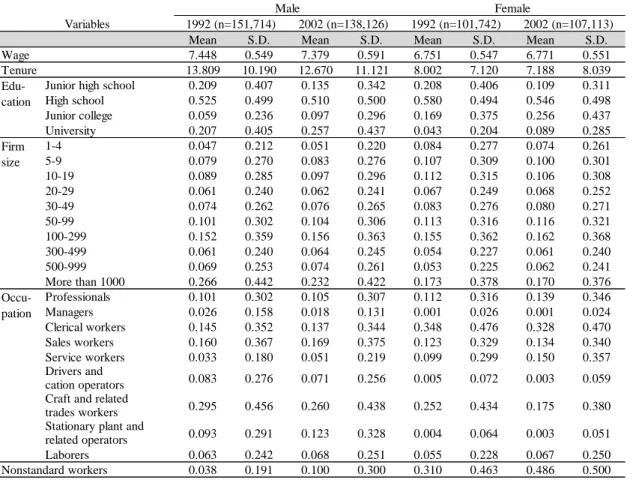
category of nonstandard workers. We analyze the data separately by gender. The descriptive statistics of these dependent and independent variables are shown in Table 1.
Table 1. Means and S.D.s of Variables
We use the Herfindahl index (HI), labor productivity, and union density as
industry-level variables.7) The HI was sourced from the Japan Industrial
Productivity (JIP) database 2006 (Research Institute of Economy, Trade and Industry, 2006). This index is defined as the sum of the squared market share of all firms within the industry. As it is calculated based on the information of Japanese domestic market, it represents domestic market concentration. A smaller number means a less concentrated market, and a larger number, a more concentrated market. As the JIP database offers the data for 1996 and 2001 only, we use the 1996 data for our 1992 survey data and the 2001 data for our 2002 survey data. The measure of labor productivity comes from the Financial Statements of Corporations by Industry. This is defined as value added per
Mean S.D. Mean S.D. Mean S.D. Mean S.D.
Wage 7.448 0.549 7.379 0.591 6.751 0.547 6.771 0.551
Tenure 13.809 10.190 12.670 11.121 8.002 7.120 7.188 8.039
Junior high school 0.209 0.407 0.135 0.342 0.208 0.406 0.109 0.311
High school 0.525 0.499 0.510 0.500 0.580 0.494 0.546 0.498 Junior college 0.059 0.236 0.097 0.296 0.169 0.375 0.256 0.437 University 0.207 0.405 0.257 0.437 0.043 0.204 0.089 0.285 1-4 0.047 0.212 0.051 0.220 0.084 0.277 0.074 0.261 5-9 0.079 0.270 0.083 0.276 0.107 0.309 0.100 0.301 10-19 0.089 0.285 0.097 0.296 0.112 0.315 0.106 0.308 20-29 0.061 0.240 0.062 0.241 0.067 0.249 0.068 0.252 30-49 0.074 0.262 0.076 0.265 0.083 0.276 0.080 0.271 50-99 0.101 0.302 0.104 0.306 0.113 0.316 0.116 0.321 100-299 0.152 0.359 0.156 0.363 0.155 0.362 0.162 0.368 300-499 0.061 0.240 0.064 0.245 0.054 0.227 0.061 0.240 500-999 0.069 0.253 0.074 0.261 0.053 0.225 0.062 0.241 More than 1000 0.266 0.442 0.232 0.422 0.173 0.378 0.170 0.376 Professionals 0.101 0.302 0.105 0.307 0.112 0.316 0.139 0.346 Managers 0.026 0.158 0.018 0.131 0.001 0.026 0.001 0.024 Clerical workers 0.145 0.352 0.137 0.344 0.348 0.476 0.328 0.470 Sales workers 0.160 0.367 0.169 0.375 0.123 0.329 0.134 0.340 Service workers 0.033 0.180 0.051 0.219 0.099 0.299 0.150 0.357 Drivers and cation operators Craft and related trades workers Stationary plant and related operators Laborers 0.063 0.242 0.068 0.251 0.055 0.228 0.067 0.250 Nonstandard workers 0.038 0.191 0.100 0.300 0.310 0.463 0.486 0.500 Firm size Edu-cation Male Female 1992 (n=151,714) 2002 (n=138,126) 1992 (n=101,742) 2002 (n=107,113) Variables 0.072 0.003 0.059 0.295 Occu-pation 0.456 0.260 0.438 0.252 0.434 0.175 0.380 0.083 0.276 0.071 0.256 0.005 0.064 0.003 0.051 0.093 0.291 0.123 0.328 0.004
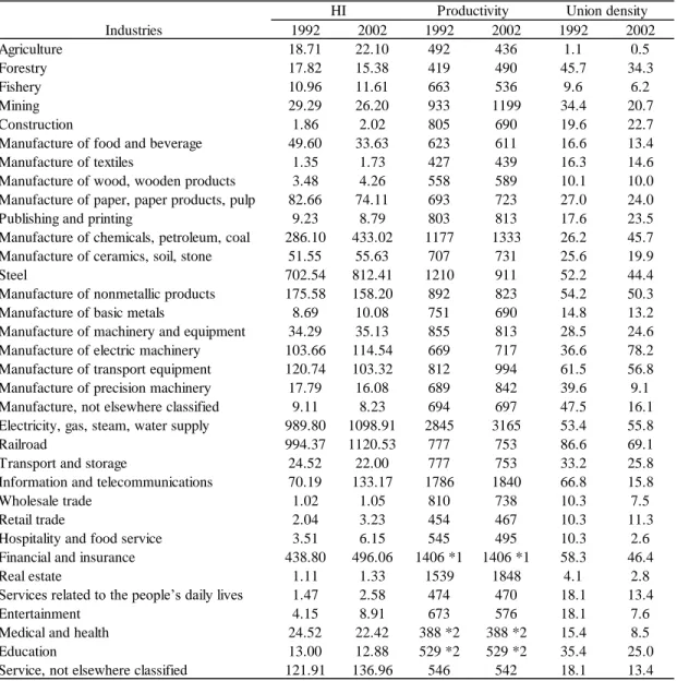
employee in units of CNY 10,000. Data for union density are taken from the Basic Survey on Labour Unions. Union density is defined as the ratio of union members to nonunion members in each industry. These industry-level variables are shown in Table 2.8)
Table 2. Industry-Level Variables
*1 Data from the Basic Survey on Business Activity in 2002. *2 Data in 2004. Analyses
Using the analytical model, data, and variables, we conduct the following two analyses. First, we estimate industry wage premiums at several quantiles using
Industries 1992 2002 1992 2002 1992 2002 Agriculture 18.71 22.10 492 436 1.1 0.5 Forestry 17.82 15.38 419 490 45.7 34.3 Fishery 10.96 11.61 663 536 9.6 6.2 Mining 29.29 26.20 933 1199 34.4 20.7 Construction 1.86 2.02 805 690 19.6 22.7
Manufacture of food and beverage 49.60 33.63 623 611 16.6 13.4 Manufacture of textiles 1.35 1.73 427 439 16.3 14.6 Manufacture of wood, wooden products 3.48 4.26 558 589 10.1 10.0 Manufacture of paper, paper products, pulp 82.66 74.11 693 723 27.0 24.0 Publishing and printing 9.23 8.79 803 813 17.6 23.5 Manufacture of chemicals, petroleum, coal 286.10 433.02 1177 1333 26.2 45.7 Manufacture of ceramics, soil, stone 51.55 55.63 707 731 25.6 19.9
Steel 702.54 812.41 1210 911 52.2 44.4
Manufacture of nonmetallic products 175.58 158.20 892 823 54.2 50.3 Manufacture of basic metals 8.69 10.08 751 690 14.8 13.2 Manufacture of machinery and equipment 34.29 35.13 855 813 28.5 24.6 Manufacture of electric machinery 103.66 114.54 669 717 36.6 78.2 Manufacture of transport equipment 120.74 103.32 812 994 61.5 56.8 Manufacture of precision machinery 17.79 16.08 689 842 39.6 9.1 Manufacture, not elsewhere classified 9.11 8.23 694 697 47.5 16.1 Electricity, gas, steam, water supply 989.80 1098.91 2845 3165 53.4 55.8
Railroad 994.37 1120.53 777 753 86.6 69.1
Transport and storage 24.52 22.00 777 753 33.2 25.8 Information and telecommunications 70.19 133.17 1786 1840 66.8 15.8
Wholesale trade 1.02 1.05 810 738 10.3 7.5
Retail trade 2.04 3.23 454 467 10.3 11.3
Hospitality and food service 3.51 6.15 545 495 10.3 2.6 Financial and insurance 438.80 496.06 1406 *1 1406 *1 58.3 46.4
Real estate 1.11 1.33 1539 1848 4.1 2.8
Services related to the people’s daily lives 1.47 2.58 474 470 18.1 13.4
Entertainment 4.15 8.91 673 576 18.1 7.6
Medical and health 24.52 22.42 388 *2 388 *2 15.4 8.5
Education 13.00 12.88 529 *2 529 *2 35.4 25.0
Service, not elsewhere classified 121.91 136.96 546 542 18.1 13.4 HI Productivity Union density
UQR analysis. Second, we estimate UQR models including industry-level variables instead of dummy variables for industry, and we examine the relationship between industry-level variables and wages at each quantile.
Analysis 1: Industry Wage Premiums at Each Quantile
First, we examine whether and in what way working in specific industries gives workers wage advantages at different points in the wage distribution. We estimate the following Model (1):
𝑅𝐼𝐹(𝑦; 𝑄𝜏) = 𝛽[𝜏]0+ ∑ 𝛽[𝜏]𝑗𝑋𝑗
𝑗 + ∑ 𝛼𝑘 [𝜏]𝑘𝐼𝑘+ 𝜀[𝜏]𝑖,
・・・Model (1)
where I is the set of dummy variables for industry and X is the set of independent
variables other than industry.
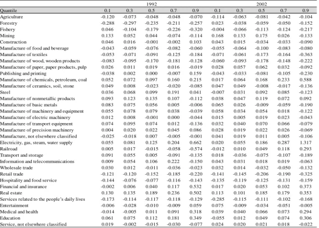
We estimate this UQR model of wage separately by gender and the two years, 1992 and 2002. Using the coefficients of industry dummy variables obtained from these models, we calculate industry wage premiums at each quantile, where the mean of wage premiums is set to zero in each quantile and each year. Although the UQR model can be estimated at any quantile, the wage premiums at quantile 0.1, 0.3, 0.5, 0.7, and 0.9 are shown in Table 3 (male) and Table 4 (female) because of space constraints.
Table 3. Industry Wage Premiums at Quantiles (Male) Quantile 0.1 0.3 0.5 0.7 0.9 0.1 0.3 0.5 0.7 0.9 Agriculture -0.120 -0.073 -0.048 -0.048 -0.070 -0.114 -0.063 -0.081 -0.042 -0.104 Forestry -0.288 -0.297 -0.235 -0.211 -0.257 0.023 -0.038 -0.059 -0.050 -0.152 Fishery 0.046 -0.104 -0.179 -0.226 -0.320 -0.004 -0.066 -0.113 -0.124 -0.217 Mining 0.133 0.052 0.044 -0.074 -0.114 0.168 0.133 0.175 0.026 -0.133 Construction 0.046 0.016 -0.001 -0.002 0.103 0.043 0.015 -0.034 -0.033 -0.090 Manufacture of food and beverage -0.043 -0.059 -0.076 -0.082 -0.060 -0.055 -0.064 -0.100 -0.083 -0.080 Manufacture of textiles -0.053 -0.071 -0.091 -0.125 -0.184 -0.071 -0.061 -0.173 -0.164 -0.363 Manufacture of wood, wooden products -0.083 -0.095 -0.170 -0.181 -0.128 -0.060 -0.093 -0.178 -0.148 -0.222 Manufacture of paper, paper products, pulp 0.026 0.011 0.019 0.016 -0.019 0.028 0.057 0.062 0.032 -0.092 Publishing and printing -0.038 0.002 0.000 -0.007 0.159 -0.043 -0.033 -0.081 -0.105 -0.230 Manufacture of chemicals, petroleum, coal 0.052 0.072 0.097 0.160 0.215 0.017 0.064 0.168 0.233 0.588 Manufacture of ceramics, soil, stone 0.049 0.008 -0.023 -0.020 -0.085 0.047 0.049 -0.008 -0.017 -0.136 Steel 0.036 0.068 0.099 0.191 0.041 -0.007 0.031 0.092 0.085 -0.123 Manufacture of nonmetallic products 0.093 0.123 0.135 0.107 -0.112 0.038 0.047 0.119 0.072 0.092 Manufacture of basic metals 0.083 0.075 0.056 0.005 -0.006 0.065 0.026 -0.009 -0.059 -0.190 Manufacture of machinery and equipment 0.055 0.078 0.079 0.038 -0.039 0.058 0.034 0.054 0.018 -0.122 Manufacture of electric machinery 0.012 0.008 -0.001 0.000 -0.044 0.015 0.005 0.019 0.023 -0.043 Manufacture of transport equipment 0.074 0.095 0.074 0.012 -0.136 0.032 0.040 0.070 0.066 -0.079 Manufacture of precision machinery 0.004 0.020 0.022 0.045 0.086 0.028 0.019 0.022 0.026 -0.069 Manufacture, not elsewhere classified -0.025 -0.018 0.007 -0.005 -0.001 0.041 0.019 0.011 0.005 -0.106 Electricity, gas, steam, water supply 0.055 0.081 0.125 0.204 0.662 0.020 0.055 0.186 0.287 1.317 Railroad 0.005 0.017 -0.015 -0.058 -0.574 -0.012 0.010 0.049 0.118 0.293 Transport and storage 0.091 0.055 0.005 -0.091 -0.135 0.018 -0.036 -0.075 -0.107 -0.189 Information and telecommunications 0.009 0.054 0.106 0.222 -0.150 0.043 0.031 0.018 0.019 -0.063 Wholesale trade 0.030 0.012 -0.011 -0.036 -0.023 0.032 0.014 -0.032 -0.050 -0.132 Retail trade -0.121 -0.120 -0.152 -0.185 -0.220 -0.141 -0.145 -0.206 -0.190 -0.325 Hospitality and food service -0.144 -0.076 -0.077 -0.116 -0.143 -0.135 -0.119 -0.125 -0.131 -0.159 Financial and insurance -0.002 0.006 0.040 0.117 0.532 0.017 0.020 0.053 0.102 0.373 Real estate 0.130 0.135 0.189 0.236 0.502 0.113 0.101 0.185 0.179 0.353 Services related to the people’s daily lives -0.173 -0.114 -0.117 -0.118 -0.129 -0.285 -0.115 -0.111 -0.102 -0.168 Entertainment -0.006 -0.028 -0.010 -0.009 0.059 0.075 -0.009 -0.034 -0.051 -0.005 Medical and health -0.014 -0.005 0.011 0.091 0.318 0.039 0.040 0.066 0.073 0.294 Education 0.061 0.075 0.112 0.181 0.349 -0.055 0.012 0.049 0.074 0.306 Service, not elsewhere classified 0.019 -0.002 -0.015 -0.030 -0.077 0.024 0.020 0.021 0.018 -0.022
2002 1992
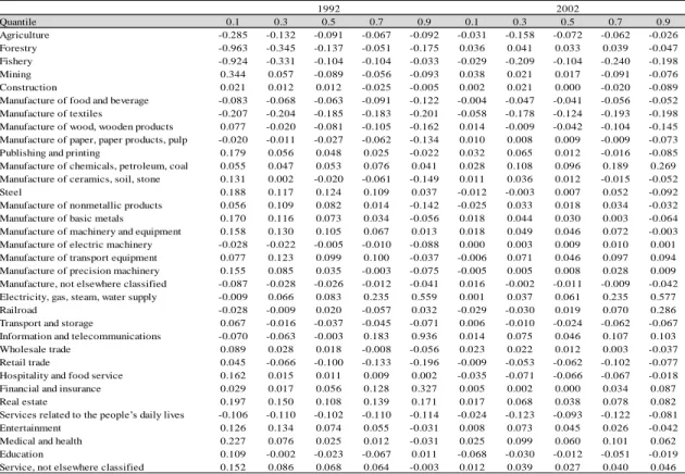
Table 4. Industry Wage Premiums at Quantiles (Female)
Tables 3 and 4 show that electricity, gas, heat, and water supply, manufacture of chemicals, petroleum, and coal products, real estate, and finance and insurance are industries with higher wage premiums. On the other hand, retail trade, services related to the people’s daily lives, manufacture of textiles, manufacture of wood and wooden products, fishery, and forestry are industries with lower wage premiums.
Tables 3 and 4 demonstrate the following four findings. First, wage premiums and penalties at higher quantiles tend to be greater than those at lower quantiles. For example, for male workers, the wage premiums of the finance and insurance industry at quantile 0.9 were 0.532 in 1992 and 0.373 in 2002, whereas those at quantile 0.1 were -0.002 in 1992 and 0.017 in 2002. The wage premiums of electricity, gas, heat, and water supply at quantile 0.9 were 0.662 in 1992 and 1.317 in 2002, and those at quantile 0.1 were 0.055 in 1992 and 0.020 in 2002. This means that employees located at the top end of the distribution received higher industry wage premiums than those at the bottom end of the distribution.
Second, industry wage premiums and penalties tended to be greater for male
workers than for female workers.9) For example, the wage premiums of
Quantile 0.1 0.3 0.5 0.7 0.9 0.1 0.3 0.5 0.7 0.9 Agriculture -0.285 -0.132 -0.091 -0.067 -0.092 -0.031 -0.158 -0.072 -0.062 -0.026 Forestry -0.963 -0.345 -0.137 -0.051 -0.175 0.036 0.041 0.033 0.039 -0.047 Fishery -0.924 -0.331 -0.104 -0.104 -0.033 -0.029 -0.209 -0.104 -0.240 -0.198 Mining 0.344 0.057 -0.089 -0.056 -0.093 0.038 0.021 0.017 -0.091 -0.076 Construction 0.021 0.012 0.012 -0.025 -0.005 0.002 0.021 0.000 -0.020 -0.089
Manufacture of food and beverage -0.083 -0.068 -0.063 -0.091 -0.122 -0.004 -0.047 -0.041 -0.056 -0.052 Manufacture of textiles -0.207 -0.204 -0.185 -0.183 -0.201 -0.058 -0.178 -0.124 -0.193 -0.198 Manufacture of wood, wooden products 0.077 -0.020 -0.081 -0.105 -0.162 0.014 -0.009 -0.042 -0.104 -0.145 Manufacture of paper, paper products, pulp -0.020 -0.011 -0.027 -0.062 -0.134 0.010 0.008 0.009 -0.009 -0.073
Publishing and printing 0.179 0.056 0.048 0.025 -0.022 0.032 0.065 0.012 -0.016 -0.085
Manufacture of chemicals, petroleum, coal 0.055 0.047 0.053 0.076 0.041 0.028 0.108 0.096 0.189 0.269 Manufacture of ceramics, soil, stone 0.131 0.002 -0.020 -0.061 -0.149 0.011 0.036 0.012 -0.015 -0.052
Steel 0.188 0.117 0.124 0.109 0.037 -0.012 -0.003 0.007 0.052 -0.092
Manufacture of nonmetallic products 0.056 0.109 0.082 0.014 -0.142 -0.025 0.033 0.018 0.034 -0.032 Manufacture of basic metals 0.170 0.116 0.073 0.034 -0.056 0.018 0.044 0.030 0.003 -0.064 Manufacture of machinery and equipment 0.158 0.130 0.105 0.067 0.013 0.018 0.049 0.046 0.072 -0.003 Manufacture of electric machinery -0.028 -0.022 -0.005 -0.010 -0.088 0.000 0.003 0.009 0.010 0.001 Manufacture of transport equipment 0.077 0.123 0.099 0.100 -0.037 -0.006 0.071 0.046 0.097 0.094 Manufacture of precision machinery 0.155 0.085 0.035 -0.003 -0.075 -0.005 0.005 0.008 0.028 0.009 Manufacture, not elsewhere classified -0.087 -0.028 -0.026 -0.012 -0.041 0.016 -0.002 -0.011 -0.009 -0.042 Electricity, gas, steam, water supply -0.009 0.066 0.083 0.235 0.559 0.001 0.037 0.061 0.235 0.577
Railroad -0.028 -0.009 0.020 -0.057 0.032 -0.029 -0.030 0.019 0.070 0.286
Transport and storage 0.067 -0.016 -0.037 -0.045 -0.071 0.006 -0.010 -0.024 -0.062 -0.067 Information and telecommunications -0.070 -0.063 -0.003 0.183 0.936 0.014 0.075 0.046 0.107 0.103
Wholesale trade 0.089 0.028 0.018 -0.008 -0.056 0.023 0.022 0.012 0.003 -0.037
Retail trade 0.045 -0.066 -0.100 -0.133 -0.196 -0.009 -0.053 -0.062 -0.102 -0.077
Hospitality and food service 0.162 0.015 0.011 0.009 0.002 -0.035 -0.071 -0.066 -0.067 -0.018
Financial and insurance 0.029 0.017 0.056 0.128 0.327 0.005 0.002 0.000 0.034 0.087
Real estate 0.197 0.150 0.108 0.139 0.171 0.017 0.068 0.038 0.078 0.082
Services related to the people’s daily lives -0.106 -0.110 -0.102 -0.110 -0.114 -0.024 -0.123 -0.093 -0.122 -0.081
Entertainment 0.126 0.134 0.074 0.055 -0.031 0.008 0.073 0.045 0.026 -0.042
Medical and health 0.227 0.076 0.025 0.012 -0.031 0.025 0.099 0.060 0.101 0.062
Education 0.109 -0.002 -0.023 -0.067 0.011 -0.068 -0.030 -0.012 -0.051 -0.019
Service, not elsewhere classified 0.152 0.086 0.068 0.064 -0.003 0.012 0.039 0.027 0.040 0.046
manufacture of chemicals at quantile 0.9 were 0.215 in 1992 and 0.588 in 2002 for male workers, but they were 0.041 in 1992 and 0.269 in 2002 for female workers. On the other hand, the wage penalties of retail trade at quantile 0.1 were -0.121 in 1992 and -0.141 in 2002 for males and 0.045 in 1992 and -0.009 in 2002 for females. The wage penalties of hospitality and food service at quantile 0.1 were -0.144 in 1992 and -0.135 in 2002 for males and 0.162 in 1992 and -0.035 in 2002 for females.
The third finding is that, among male workers at the top end of the distribution, industry wage premiums and penalties tended to increase between 1992 and 2002, and inter-industry wage differentials seemed to increase. For example, the wage premium of manufacture of chemicals at quantile 0.9 was 0.215 in 1992, but it became 0.588 in 2002. Also, the wage premium of electricity, gas, heat, and water supply was 0.662 in 1992, but it was 1.317 in 2002. On the other hand, the wage penalties of manufacture of textiles at quantile 0.9 were -0.184 in 1992 and -0.363 in 2002. Those of manufacture of wooden products were -0.128 in 1992 and -0.222 in 2002.
Finally, among female workers at the bottom and top ends of the distribution, industry wage premiums and penalties tended to decrease between 1992 and 2002, and inter-industry wage differentials seemed to decrease. For example, the wage premiums of the steel industry at quantile 0.1 were 0.188 in 1992 and -0.012 in 2002. Those of manufacture of machinery and equipment were 0.158 in 1992 and 0.018 in 2002. On the other hand, the wage premiums of finance and insurance at quantile 0.9 were 0.327 in 1992 and 0.087 in 2002. Those of real estate were 0.171 in 1992 and 0.082 in 2002. Also, the wage penalties of retail trade at quantile 0.9 were -0.196 in 1992 and -0.077 in 2002.
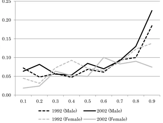
Next, we calculate the weighted adjusted standard deviation (WASD) to summarize the overall variability in industry wages (Figure 1). The WASD is a measure developed by Krueger and Summers (1988) and has been used previously (Katz & Summers, 1989; Tachibanaki & Ota, 1992). This measure considers the numbers of employees in each industry and the upwardly biased estimate of the standard deviation of coefficients. We use coefficients obtained from the UQR models to see whether inter-industry wage differences differ across the wage distribution. We calculate the WASD using coefficients at nine quantiles dividing the wage distribution into equal groups.
Figure 1. Inter-Industry Wage Differentials Measured by the Weighted Adjusted
Standard Deviation (WASD)
The result displayed in Figure 1 underscores the changing pattern of industry wage premiums as discussed above. According to Figure 1, inter-industry wage differentials are greater at the top end of the distribution, especially for male workers. Furthermore, inter-industry wage differentials tend to have increased between 1992 and 2002 for males at the top end of the distribution. For female workers, inter-industry wage differentials decreased at almost every quantile except for quantile 0.6.
In sum, our analyses indicate that there are substantial inter-industry wage differentials, especially among male workers at the top end of the wage distribution, and these wage differences increased for males between 1992 and 2002. Compared to males, inter-industry wage differentials are not so great for female workers, and they decreased between 1992 and 2002.
This suggests that there are structural processes of distributing wages to employees, which are not explained by the competitive labor market model. Specifically, these results indicate the possibility that economic environments faced by firms in each industry are important for employees’ wages, and these environmental advantages generate profits, which are then shared by workers.
0.00 0.05 0.10 0.15 0.20 0.25 0.1 0.2 0.3 0.4 0.5 0.6 0.7 0.8 0.9 1992 (Male) 2002 (Male) 1992 (Female) 2002 (Female)
In the next subsection, we identify the factors determining wage differences between industries.
Analysis 2: Determinants of inter-industry Wage Differentials
We estimate the URQ model using the following industry-level variables: the HI, labor productivity (LPROD), and union density (UNION), instead of dummy variable for industry in Model (1). Model (2) is presented as follows:
𝑅𝐼𝐹(𝑦; 𝑄𝜏) = 𝛽[𝜏]0+ ∑ 𝛽[𝜏]𝑗𝑋𝑗 𝑗
+ 𝜒[𝜏]𝐻𝐼 + 𝜆[𝜏]𝐿𝑃𝑅𝑂𝐷 + 𝜇[𝜏]𝑈𝑁𝐼𝑂𝑁 + 𝜀[𝜏]𝑖
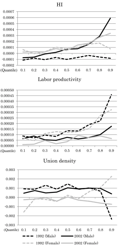
・・・Model (2) The coefficients of these three industry-level variables at nine quantiles obtained from Model (2) are displayed in Figure 2. Figure 2 shows the following four findings. First, except for the effect of HI for male workers in 1992, both HI and the labor productivity have significant positive effects on wages, especially at the top end of the distribution. This suggests that an industry’s high market concentration and high labor productivity increase wages of employees, and these industry wage premiums are shared by employees at the top end of the distribution. We also find that this rent-sharing occurred through mechanisms other than workers’ collective bargaining because the coefficients of the HI and productivity remain significant after controlling for union density.
HI
Labor productivity
Union density
Figure 2. Coefficients of Industry-Level Variables on Wages
-0.0002 -0.0001 0.0000 0.0001 0.0002 0.0003 0.0004 0.0005 0.0006 0.0007 0.1 0.2 0.3 0.4 0.5 0.6 0.7 0.8 0.9 0.00000 0.00005 0.00010 0.00015 0.00020 0.00025 0.00030 0.00035 0.00040 0.00045 0.00050 0.1 0.2 0.3 0.4 0.5 0.6 0.7 0.8 0.9 -0.003 -0.002 -0.001 0.000 0.001 0.002 0.003 0.1 0.2 0.3 0.4 0.5 0.6 0.7 0.8 0.9 1992 (Male) 2002 (Male) 1992 (Female) 2002 (Female) (Quantile) (Quantile) (Quantile)
Second, union density has a significant effect on wages, but the directions of the effects differ between males and females. For male workers, union density has significant positive effects at almost all quantiles except for a negative effect at the top end of the distribution in 1992. This means that male employees in industries with high union density are paid higher wages. On the other hand, union density tends to have negative effects at each quantile for female workers. This means that unions do not help female workers earn higher wages. Also, we note that the effects of union density changed for female workers between 1992 and 2002. Union density had positive effects at top end of the distribution in 1992, but it had negative effects in 2002.
Contrary to these results for union density, we note clearer changing patterns of the effects of the HI and labor productivity. Thus, our third finding is that the effects of the HI increased between 1992 and 2002, especially at the top end of the distribution. The coefficient changed significantly at quantile 0.9 for male workers. In 2002, the coefficient of the HI at quantile 0.9 was 0.00059. This means that, for example, the wage of male workers in the electricity, gas, heat, and water supply industry (HI = 1098.91) was 1.9 times higher than that of male workers in retail trade (HI = 3.23) at quantile 0.9 in 2002. On the other hand, the effect of the HI was negative and stayed between -0.0001 and 0 in 1992. This negative effect means that working in industries with high market concentrations was not advantageous for male workers in 1992. However, considering a model that includes only the HI as the industry-level independent variable, the effect of the HI was significant and positive in 1992 as well as in 2002. The effect of the HI was negative in the model including both HI and labor productivity in 1992. This means that male workers in industries with high market concentrations were paid higher, but this was because these industries were more productive.
Finally, we find that the effects of labor productivity on wages decreased, especially at the top end of the distribution between 1992 and 2002. In 1992, the coefficient of labor productivity at quantile 0.9 was 0.00046 for male workers. This means that the wage of male workers in electricity, gas, heat, and water supply (LPROD = 2845) was 3.0 times higher than that of male workers in retail trade (LPROD = 454) at quantile 0.9 in 1992. However, this high wage advantage decreased between 1992 and 2002. In 2002, the coefficient at quantile 0.9 was 0.00017, which means that the estimated wage advantage of male workers in the electricity, gas, heat, and water supply industry was 1.6 times higher than that of male workers in retail trade.
Discussion
findings. First, there are substantial inter-industry wage differentials, especially among male workers at the top end of the wage distribution, and these wage differentials increased between 1992 and 2002. Compared to male workers, wage differences between industries among female workers did not vary across the wage distribution, and these inter-industry wage differentials decreased between 1992 and 2002. Second, market concentration (HI), labor productivity, and union density tended to have significant and positive effects on wages at different quantiles except for the negative effect of union density on wages for female workers. Also, the effects of market concentration and labor productivity tended to be greater at the top end of the wage distribution. Third, the effects of market concentration on wages increased, whereas the effects of labor productivity decreased between 1992 and 2002, especially at the top end of the distribution.
We discuss these findings in the next subsection, focusing on economic segmentation and rent-sharing as explanations for inter-industry wage differentials. After examining these two processes, we discuss the changing trends during the 1990s.
Economic Segmentation and Rent-sharing as Explanations for Inter-industry Wage Differentials
The results suggest that there are structural processes of distributing wages to employees, namely, economic segmentation and rent-sharing, in the labor market. In terms of economic segmentation, we found that industries’ high market concentrations and labor productivity are related to higher wages of both male and female employees. These results demonstrate that firms in different industries deal with different economic environments to conduct their business, and the environmental advantages pertaining to each industry generate profits, which become sources of high wages for the employees in these industries. Although there are some changing trends, as discussed below, the positive effects of these two factors on wages basically remained unchanged during the 1990s.
In terms of rent-sharing, we observe the following two findings. First,
industries’ high union density is related to high wages for male workers.10) This
suggests that rent-sharing is prompted by workers’ great bargaining power. However, the effects differ between genders. Union density had negative effects at most quantiles for female workers except for its positive effect at the top end of the wage distribution in 1992. This fact could reflect the Japanese collective bargaining system that typically represents the interests of full-time male workers. In Japan, unions are mostly formed within firms. Therefore, it is said that unions maintain a cooperative attitude towards employers. This is possible because unions focus on representing a specific group of employees, namely, full-time male workers. In 1992, union density had positive effects for females at the top end of
the distribution, which means that high union density was advantageous for only a small portion of female workers. However, this positive effect disappeared in 2002, and furthermore, high union density was related to lower wages for female workers. This suggests that a union might sacrifice the interests of female workers to increase male workers’ wages.
The second finding is that rent-sharing is not completely determined by workers’ bargaining power. Market concentration and labor productivity, which measure economic segmentation, have substantial effects on wages even after controlling for union density. Previous studies suggest that employers could share industry rents with their employees for a number of reasons, such as reducing resignations and turnover, decreasing incentives to shirk work, and/or raising the average quality of the workforce (Genrea et al., 2011). Although it is difficult to directly observe such (often unwritten) contracts between employers and employees, our results show that such an agreement to share industry rents between employers and workers may, in fact, exist. The following result supplements this argument: industry wage premiums are shared, especially by male workers located at the top end of the distribution. This also means that in high wage industries, wage inequality within industries is higher among male workers. Accordingly, we would argue that employers in high wage industries treat male workers differently and implement wage differentials among them to provide employees incentives.
Changes in the Economic Segmentation Structure during the 1990s
As discussed above, these employment strategies in high wage industries could be feasible because of economic segmentation. However, our results show that the source for higher wages, in other words, the structure of economic segmentation, changed during the 1990s. Between 1992 and 2002, the effect of market concentration on wages increased, whereas the effect of labor productivity decreased.
Why, then, did these changes take place during the 1990s? First, in terms of the effect of labor productivity on wages, in 1992, firms in profitable industries could afford to pay higher wages to employees, and the fruits of labor were distributed to workers, especially those at the top end of the distribution. However, by 2002, the effect of labor productivity on wages had decreased. This might reflect a change in employment strategies adopted by firms. According to Noda and Abe (2010), labor share has shown a downward trend since the mid-1990s in Japan, and this decreasing trend emerged when firms increased productivity. The authors also indicated that wage level varies depending on how firms raise financing, and wages are set to lower levels at firms that rely on the capital market to raise these funds. Since the 1990s, many firms have changed their way of raising funds, and
therefore, firms’ profits might have gone to stockholders and internal reserve and not to employees. We argue that because of these changes, firms in profitable industries also might have stopped paying higher wages to employees.
Next, we discuss why the effect of domestic market concentration on wages increased during the 1990s. The first point to note here is that every company faces severe competition in domestic and internal markets. Many companies try to cut labor costs, and companies even in highly profitable industries may not share their profits with their workers. However, companies in oligopolistic industries could afford to pay higher wages to workers because of the following reason: competitive environments would change very quickly, influencing firms’ profits. Thus, it has become difficult for firms to predict future profits. On the other hand, firms in industries with high domestic market concentration could anticipate future profits more easily than firms in other industries. We suggest that this is one reason why domestic market concentration is highly advantageous for workers.
Interestingly, these changes in the structure of economic segmentation caused different changes in the patterns of inter-industry wage differentials between genders: inter-industry wage differentials increased for male workers and decreased for female workers during the 1990s.
In considering these differences it is useful to reflect on some recent studies on the American labor market that have reported that inter-industry wage differentials have decreased since the 1990s. Kim and Sakamoto (2008) interpreted this result as suggesting that firms no longer pass on a portion of their rents to broad groups of workers. Morgan and Tang (2007) explained the decreasing trend in inter-industry wage differentials by arguing that it is because people at the bottom of the class structure have been disproportionately harmed by changes in employment relations. We found a similar trend among females but not among males in Japan.
Our results reveal that the effect of labor productivity on wages decreased for females more considerably than for males at the bottom end and center of the wage distribution. On the other hand, the effect of market concentration on wages increased for male workers more substantially than female workers. Workers’ bargaining power measured by high union density did not help female workers earn higher wages. We conclude that firms no longer pass on a portion of their rents especially to female workers. These changing trends generated rent destruction for female workers and rent rising for male workers between 1992 and 2002.
Conclusion
This paper examined how inter-industry wage differentials changed during the 1990s in Japan using UQR analysis and the Employment Status Survey. We also utilized industry-level variables (the HI, labor productivity, and union density) to examine whether and in what way inter-industry wage differentials are explained by two structural processes of distributing wages, namely, economic segmentation and rent-sharing.
We found that inter-industry wage differentials and the relationship between industry-level variables and wages vary across the wage distribution. Specifically, inter-industry wage differentials tend to be greater at the top end of the distribution, especially for male workers, and changes during the 1990s took place at the top end of distribution. Accordingly, we argue that it is important to focus on different points in the wage distribution to study wage inequality. If we focus only on one representative value, such as the mean or median, we might overlook substantial inter-industry wage differentials and changing trends.
Our results also underline the importance of noncompetitive explanations for inter-industry wage differentials. There were substantial inter-industry wage differentials after controlling for workforce characteristics, and all of our industry-level variables showed significant effects on wages.
However, our analysis suffers from several limitations. First, information about firms is not available in our data. Although we discussed that there might be contracts causing rent-sharing between employers and employees, we could not actually observe what happens in firms. Many recent studies have used employer– employee matching data to show evidence of rent-sharing (Arai, 2003; Du Caju et al., 2011; Gannon et al., 2007; Guertzgena, 2010; Lundin & Yun, 2009). It is effective to use this kind of data to address questions about structural processes of distributing wages. Second, our data were sourced from a cross-sectional survey. Therefore, we could neither control unobserved workers’ characteristics nor examine whether the observed industry wage premiums reflected unobserved workers’ characteristics such as ability. It is important to consider possible selection biases that could influence worker allocation to specific industries. Finally, as our industry-level variables were limited, we might have overlooked
other important industry-level variables.11)
To conclude, we demonstrated substantial inter-industry wage differentials during the 1990s. In the future, we plan to examine the structural processes of distributing wages using recent data with rich information about workers, firms, and industries.
References
Arai, M. (2003). Wages, profits, and capital intensity: Evidence from matched
worker‐firm data. Journal of Labor Economics,21(3), 593–618.
Baron, J. N., & Bielby, W. T. (1984). The organization of work in a segmented
economy. American Sociological Review,49(4), 454–473.
Cabinet Office. (2009). Annual report on the Japanese economy and public finance.
[In Japanese]
Dickens, W. T., & Katz, L. F. (1987). Inter-industry wage differences and theories
of wage determination (NBER Working Paper No. 2271).
Du Caju, P., Rycx, F., & Tojerow, I. (2011). Inter-industry wage differentials: How
much does rent sharing matter? The Manchester School,79(4), 691–717.
Firpo, S., Fortin, N. M., & Lemieux, T. (2009). Unconditional quantile regressions.
Econometrica,77(3), 953–973.
Fournier, J.-M., & Koske, I. (2012). The determinants of earnings inequality -
Evidence from quantile regressions. OECD Journal: Economic Studies, 1, 7–
36.
Gannon, B., Plasman, R. Rycx, F., & Tojerow, I. (2007). Inter-industry wage differentials and the gender wage gap: Evidence from European countries.
The Economic and Social Review,38(1), 135–155.
Genrea, V., Kohn, K., & Momferatou, D. (2011). Understanding inter-industry
wage structures in the Euro area. Applied Economics,43, 1299–1313.
Gittleman, M., & Pierce, B. (2011). Inter-industry wage differentials, job content
and unobserved ability. Industrial & Labor Relations Review,64(2), 356–374.
Gittleman, M., & Wolff, E. N. (1993). International comparisons of inter-industry
wage differentials. Review of Income and Wealth,39(3), 295–312.
Guertzgena, N. (2010). Rent-sharing and collective wage contracts-evidence from
German establishment-level data. Applied Economics,42(22), 2835–2854.
Higuchi, Y. (1989). Japan’s changing wage structure: The impact of internal
factors and international competition. Journal of the Japanese and
International Economies,3, 480–499.
Kalleberg, A. L., Wallace, M., & Althauser, R. P. (1981). Economic segmentation,
worker power, and income inequality. American Journal of Sociology, 87(3),
651–683.
Katz, L. F., & Summers, L. H. (1989). Industry rents: Evidence and implications.
Brookings Papers on Economic Activity, 209–290.
Kim, C., & Sakamoto, A. (2008). Declining inter-industry wage dispersion in the US. Social Science Research,37(4), 1081–1101.
Kim, C., & Sakamoto, A. (2010). Assessing the consequences of declining unionization and public-sector employment: A density-function decomposition
of rising inequality from 1983 to 2005. Work and Occupations,37(2), 119–161. Kosai, Y., & Ito, Y. (2000). Income distribution in the technological innovation and
globalization: Changes in wage inequality. FRI Research Report, 72. [In
Japanese]
Krueger, A. B., & Summers, L. H. (1988). Efficiency wages and the inter-industry
wage structure. Econometrica,56(2), 259–293.
Lundin, N., & Yun, L. (2009). International trade and inter-industry wage
structure in Swedish manufacturing: Evidence from matched
employer-employee data. Review of International Economics,17(1), 87–102.
Morgan, S. L., & Tang, Z. (2007). Social class and workers’ rent, 1983-2001.
Research in Social Stratification and Mobility,25(4), 273–293.
Noda, T., & Abe, M. (2010). Labor share and wage decline. In Y. Higuch, &
Economic and Social Research Institute of the Cabinet Office (Eds.), The
labor market and income distribution (pp. 3–45). Keio University Press. [In Japanese]
Ota, K. (2005). Income and wage inequality in Japan. Labor Research,436, 38–48.
[In Japanese]
Ota, K. (2010). Wage inequality between individuals, organization sizes, and industries. In Y. Higuch, & Economic and Social Research Institute of the
Cabinet Office (Eds.), The labor market and income distribution (pp. 319–
368). Keio University Press. [In Japanese]
Otake, F. (1994). Income and wealth distribution in the 1980s. The Economic
Studies Quarterly,45(5), 385–402. [In Japanese]
Research Institute of Economy, Trade and Industry. (2006). Japan Industrial Productivity Database 2006. Retrieved April 4, 2014, from
http://www.rieti.go.jp/jp/database/d05.html.
Tachibanaki, T., & Ota, S. (1992). Inter-industry wage differentials in Japan. In T.
Tachibanaki (Ed.), Assessment, promotion and wage determination (pp. 181–
205). Yuhikaku. [In Japanese]
Ueshima, Y., & Funaba, T. (1993). Determinants of inter-industry wage
differentials. The Journal of Japan Economic Research, 24, 42–72. [In
Japanese]
Weeden, K. A., & Grusky, D. B. (2014). Inequality and market failure. American
Behavioral Scientist,58(3), 473–491. Notes
1) According to Ota (2005), the Basic Survey on Wage Structure covers only 45
percent of male employees.
economic segmentation are not appropriate. However, the existence of inter-industry wage differentials shows that industry type is an important factor that determines the wage distribution.
3) Unlike Moran and Tang (2007), we do not use the class category to examine
selective rent destruction because class category is not available in our data.
4) Our data are provided by the National Statistics Center. The data are
processed to improve anonymity. The respondents are randomly resampled using 80 percent of the original response data. Unusual households, such as households with more than eight people or households with more than three people of the same age, are deleted to prevent them from being identified.
5) The variable of hourly wage is calculated using the variables of annual
wage and weekly working hours, which are originally categorical variables. These categorical variables are transformed into continuous variables using the median of each category. Because the exact continuous values of wage and working hours are not available, there might be some measurement errors.
6) We estimate the Gini coefficient and find that overall wage inequality
increased between 1992 and 2002 for males (Gini: 0.0412→0.0446). On the other hand, wage inequality was almost stable for females (Gini: 0.0450→0.0448).
7) We do not include the variable of capital–labor intensity in our model
because capital–labor intensity is highly correlated with labor productivity.
8) The industrial classifications of the three surveys used for industry-level
variables do not correspond directly to our classifications. For example, we have one category for “electricity, gas, heat, and water supply” in the Employment Status Survey, but the JIP database has one category each for these industries. Where there are more than two categories in the JIP database and only one category in our data, we use the average value of these corresponding categories. Also, as no category corresponds to “service, not elsewhere classified” in the JIP database, we use the average values of all service industries for the category. The industrial classifications of the Financial Statements of Corporations are broader than those of the Employment Status Survey. For example, as the value for the railroad industry is not available in the Financial Statements of Corporations, we substitute the value of the transport industry for the railroad industry. Also, as data for the food service industry are not available, we use the value of the hospitality industry. As we cannot obtain a value for the financial and
insurance industry, we substitute the value for this industry with the corresponding value from the Basic Survey on Business Activity. As the values for medical and health, and education, are available for 2004 only, we use the value of 2004 for our 1992 and 2002 data.
9) However, the wage penalties of the forestry and fishery industries are
significant for female workers. This might be because there are only a few female employees in these industries, and sampling errors might be greater for these two industries than for other industries.
10) In 1992, union density had a negative effect at the top end of the
distribution for male workers. This is understandable given the fact that unions could play a role in compressing wage inequality within each workplace, and thus, high union density could lead to smaller wage inequality within industries. For example, Firpo et al. (2009) showed that the effects of union membership on wages are negative at the top end of the distribution in the United States. However, our result shows that unions no longer had such an effect in 2002.
11) Some previous studies showed that intensity of global competition is also
an important factor affecting wage differences between industries. Lundin and Yun (2009) demonstrated that industries facing intensive import competition from low-income countries have lower wage premiums.