膝 関節 軟 骨 力 学 特 性 の非 侵 襲 的 定 量 的評 価 法 に関す る研 究

Developmentsofquantitativeandnon‑invasivemethods forevaluatingmechanicalpropertyofthekneearticular cartilage

膝 関節 軟 骨 力 学 特 性 の非 侵 襲 的 定 量 的評 価 法 に関す る研 究

平 成25年1月10日 提 出

首都大学東京 大学院

人間健康科学研究科 博士後期課程 人間健康科学専攻

放 射 線 科 学 域

学修 番 号:10997601

氏 名 清 木 孝子

(指導 教 員名:古 川 顕 教 授)

博 士 学 位 論 文

Developmentsofquantitativeandnon‑invasivemethodsfor

evaluatingmechanicalpropertyofthekneearticularcartilage

膝 関節 軟 骨 力 学 特 性 の 非 侵 襲 的 定 量 的 評 価 法 に 関 す る研 究

平 成25年1,月10日 .提 出

首都 大学東京 大学院

人 間健 康科学研究科 博 士後期課程 人 間健康科学専攻

・ 放 射 線 科 学 域

学 修 番 号:10997601 氏 名:青 木 孝 子

(指 導 教 員 名:古 川 顕 教 授)

1

Contents

Overview Chapter 1

1. Bac]

prolegomenon 1 Background

1.2 Objective 1. Contribut 1.4 Approach 1. Constituti 3

ion

- Constitution

1.6 Conflict of interest Chapter 2 Mechanis

2.1 Cartilaginousstruc

Mechanism of osteoarthritis and cartilaginous relations Cartilaginous structure

2.2 Change of the articular cartilage with osteoarthritis 2.3 Evaluation of OA...

2.3.1 Initial consultation

1 2 2 2 3 3 3 4 5 5 8

2.3.2 Kellgren-Lawrence Score 2.3.3 Outerbridge classification

2.3.4 Modified Outerbridge classification using MRI

2.3.5 Quantitative cartilage imaging using MRI...

Chapter 3 Microscopic water molecule motion in the cartilage obtained

diffusion weighted images 3.1 Free diffusion...

10 11 11 12 13 14 from

3.2 Restricted diffusion

3.3 Diffusion in articular cartilage...

Chapter 4 Evaluating relation between apparent diffusion coefficient viscoelasticity of the cartilage

4.1 Introduction...

16 16 19 21 and

.. 25

4.2 Theory supported Tip 4.2.1 Spin-Lock pulse

4.2.2 Magnetization in the rotating frame

4.2.3 Tip-prepared segmented multi-shot 3D-TFE sequence 4.2.4 Behavior of the magnetization of the transient period.

4.2.5 Artifact...

4.3 Basic points of mechanical property 4.3.1 Viscoelasticity ...

4.3.2 Effect of temperature on viscoelastic behavior

25

27

27

28

30

32

33

34

34

35

4.3.3 Stress relaxation

4.4 Material and Methods 4.4.1 Subjects...

4.4.2 MR Imaging 4.4.3 ROI setting

4.4.4 Mechanical testing 4.4.5 Statistical analysis 4.5 Results ...

4.6 Discussion...

4.7 Conclusion...

Chapter 5 Evaluating relation between speed of sound and elasticity of cartilage ...

5.1 Introduction

35 37 37 37 39 41 42 43 46 49 the .. 50

5.2 Theory supporting the speed of sound measurements 5.2.1 Basic ultrasound...

5.2.2 Incidence angle and the distance

5.2.3 The transmission method measurement of speed of sound (SOS) 5.2.4 The SOS measurement by combination method...

5.3 Materials and Methods...

5.3.1 Specimen preparation 5.3.2 MRI imaging...

5.3.3 Thickness measurements of specimens 5.3.4 SOS measurements in cartilage specimens 5.3.5 Statistics

5.4 Results ...

5.4.1 Thickness measurements of specimens...

5.4.2 Comparison of SOS using transmission method and combination method . 5.5 Discussion...

5.6 Conclusions...

Chapter 6 Comparison of the speed of sound and T2 relaxation time cartilage in the assessment of its degenerative change...

6.1 Introduction...

50 52 52 54 55 57 59 59 60 61 63 64 65 65 65 67 69 of the

6.2 Materials and Methods

6.2.1 Subjects

6.2.2 MR imaging

6.2.3 Problem of applying the pulse-echo method

111

70

70

71

71

71

72

6.2.4 Applying the real-time virtual sonography (RVS)

6.2.5 Definition of the cartilage thickness 6.2.6

6.3 Results

Conclu Chapter 7

References... atistics Discus!

Conclusions

Summery

Chapter 1 Chapter 2 Chapter 3 Chapter 4 Chapter 5 Chapter 6 Acknowledgment

74 77 78 79 80 83 84 87 87 88 89 90 96 99

103

iv

Overview

変形性膝 関節症(OA)は 加 齢性 に増加 し、超 高齢化社会 において生活の質の維 持や 医療経 済 に とって深刻 な疾患 の一っ であ る。近年、OA初 期 の加療 において進行 の抑制が期待 され る 抗OA薬 が開発 され たが、OA初 期 の診 断法は確 立 されてい ないた め早期診断 は困難 で、整形 外科受診時 にはかな り進行 してい る。軟骨は主 にi:i%の 水 分 と細胞外基質で構… 成 され 、軟 骨細胞 はわず かで血 管、神経 、 リンパ 管 はな く、膝 の運動 に よる関節液 の流動 に よ り栄養 さ れ、細胞外基質 であ るコラ0ゲ ン線維 とプ ロテオ グ リカ ンが軟骨機 能 の維持 に重 要な役割 を 担 ってい る。軟 骨表層 のコラー ゲ ン線維 は関節面 と並 走 し軟骨 にかか る荷重 を支 え、プ ロテ オ グ リカンは水 分 を保 持 しク ッシ ョンの役割 を担 う。加齢 とともにコラ0ゲ ンの変性 とプ ロ テオ グ リカンの減少 が 同時 に進行 してい き、最終 的に荷重 を支 える ことができな くな り軟骨 が破壊 され る。軟骨 は修復 ・再生 され るこ とはないた め、軟骨 が変性 しOAへ 進行 してい く

と、姑息 的対症 療法の後 、最終 的 に骨切 り術 または人 工関節 置換術 の手術適応 とな るが、高 齢者で は 自立 した生活 は困難 にな る。従 って、軟骨変性 に伴 う変化 を定量評価す ることがOA 初期 の診断 に重要 であ る。

本研究 は コラーゲ ンの変性 に伴 う物理特性変化 の定量的評価 法 を考案 し、その測定精度 を 検証 した。 見かけの拡散係 数(ADC)は 含 水量 を示す とともに、吸水性 を示す と考 え、 ブタ 軟骨 を用 いて力 学試験 に よる粘 弾性 とADCの 高い相 関を確認 した。寒天 ファン トムを用 いて 基礎実験 を行 い、MRIと 超音波 を併用 した軟骨 の音速 測定法 の測定精度 を確認 した。MRIと 超音波 を併 用 した軟骨 の音速 測定法 を生体へ応用 し、ボ ランテ ィア(倫 理 申請 で承認 され 、

同意 の得 られ た者)に よる測定でT2値 と高い相 関が得 られ た。音速 はT2と 同 じ現象 を と ら えてい るこ とが示 され 、信頼性 が得 られ た。本研 究は不可能 とされ ていた生体軟骨 の非侵襲 的物理 的特性(弾 性、粘 弾性)の 測定 が可能 である ことを示 した。

1

Chapter 1 prolegomenon

1.1 Background

Osteoarthritis (OA) is a degenerative disease of cartilage that progresses slowly by erosive deterioration of articular cartilage, and develops most commonly in weight-bearing regions. Structural change of the collagen array and decrease in water content by decreased proteoglycan occur in early stage of OA, [1-3] and capacity of the load support causes decline of the elasticity by structural change of the collagen array and becomes more serious with progress of disease [4]. Since symptoms do not appear in the early stage of OA, it progresses without noticing the onset. Diagnosis in early stage and. control of progressive OA are important issue in super-graying society.

1.2 Objective

The aim of this study was to develop noninvasive in-vivo measuring methods for the

changes in the cartilage. The all studies were approved by the institutional review board.

2

1.3 Contribution

Development of new noninvasive quantitative evaluation methods assessing

mechanical property of the cartilage using MRI and/or ultrasound for early detection

and correct diagnosis of OA.

1.4 Approach

Newly developed two non-invasive quantitative evaluation methods using MRI and/or

ultrasound to assess the mechanical property of the cartilage are demonstrated and their

accuracies are discussed.

1.5 Constitution

In Chapter 2, describes basics point of OA. In Chapter 3 describes basics point of

behavior of molecules diffusion. From Chapter 4 to 9, examines newly proposed

method for assessing the elasticity, . and summarizes this article in last chapter 10.

3

1.6Conflictofinterest

ThisreserchwasconductedbyagrantfromPolcy‑basedmedicalservicesfoundation

﹁へ

寧

4

Chapter 2 Mechanism of osteoarthritis and cartilaginous relations

2.1 Cartilaginous structure

Articular cartilage is a living material composed of a relatively small number of cells known as chondrocytes surrounded by a multicomponent matrix. Approximately 70 to 85% weight of the whole tissue is water and the remainder of the tissue is composed

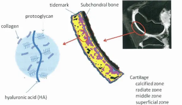
primarily of proteoglycans (PG) and collagen (Fig. 2-1). These PGs can bind or aggregate to a backbone of hyaluronic acid to form a macromolecule and account approximately 30% of the dry weight of articular cartilage. PG concentration and water content vary through the depth of the tissue. Near the articular surface, PG concentration is relatively low and the water content is highest in the tissue. In the deeper regions of the cartilage, near subchondral bone, the PG concentration is greatest and the water content is lowest. Collagen is a fibrous protein that makes up 60 to 70%

of the dry weight of the tissue. Type II is the predominant collagen in articular cartilage, although other types are present in smaller amounts. Collagen architecture varies through the depth of the tissue and the structure of articular cartilage is often

5

described in terms of four zones between the articular surface and the subchondral bone: the surface or superficial tangential zone, the intermediate or middle zone, the

deep or radiate zone, and the calcified zone. The calcified cartilage is the boundary between the cartilage and the underlying subchondral bone. The interface between the deep zone and calcified cartilage is known as the tidemark [1].

tidemark Subehond I bone

collagen

proteogl ycan

hyahhronis acid (HA)

Fig. 2-1. Sc

POO 'Try_

<?.

calcified zone radiate zone middle zone superficial zone Fig. 2-1. Schematic illustration of cartilaginous constitution

Fig. 2-2 showed electron microscopy image of cartilage and high-power scanning

electron microscopy image of deep layer. Matrix collagen within cartilage is organized

in leaflike structures that radiate from the subchondral interface in a perpendicular

6

orientation and then curve into the horizontal orientation at the articular surface (Fig.

2-3).

71i.STWAYAM

Fig. 2-2 Microstructure of cartilage

Electron microscopy image of cartilage (a) and high power electron microscopy image of the collagen network in deep layer (Radiate zone) (b). [2].

)N

•

'1

Irk711/1116 1,

- F.74:.,-Ikini

1-• hiietreAele

Ila di=

Caicrigd Sar.hcccal

Fig. 2-3 Collagen network orientation of cartilage [1]

7

2.2 Change of the articular cartilage with osteoarthritis

Osteoarthritis is classified as primary when aetiology and pathogenesis are unknown.

The known causes are mechanical or metabolic risk factors such as aberrance of the axis, haemophilia, rheumatoid and bacterial arthritis, osteochondrosis dissecans, dysplasia of the joint, injury, etc. The most common joints involved in OA are the knee joints major risks come from occupations that require repetitive bending of the joint. Obesity may be

a further factor in the development of osteoarthritis, particularly of the knee and especially in women. However, once osteoarthritis has developed, the work-related repetitive movement often makes the disorder worse [3].

Since a self-repair function is poor and neither the nerve nor the blood vessel exists in cartilage, symptoms seldom occur in the early stage of the OA as the disease

progress symptoms and deformity of the bones appear, and total knee replacement (TKR) is required at the terminal stage (Fig. 2-4).

8

(a)

Fig. 2-4 Tei

The typical case appearance (a)

Increasing grade indicates progression of C

demonstrated and graded pathologically as

superficial fibrillation, grade 2: superficial

vertical fissures extending into mid zone. a

(b) Fig. 2-4 Terminal case of OA

The typical case appearance (a), Roentgenogram of after TKR (b) [4]

Increasing grade indicates progression of OA (Fig. 2-5). The progress of the disease is demonstrated and graded pathologically as follows; grade I: uneven surface and superficial fibrillation, grade 2: superficial discontinuity and focal fibrillation, grade 3:

vertical fissures extending into mid zone, grade 4-6: destruction of the cartilage.

Grade 0 (Normal)

9

Fig. 2-5 OA cartilage pathology (Safranin 0 stain) [5].

Safranin 0 stain, original magnification x5.

2.3 Evaluation of OA

OA changes of the knee joints are diagnosed and graded either with plain radiographs using K-L scoring system and/or arthroscopy and/or MRI using Outerbridge or

modified Outerbridge classification. As a new approach, quantitative assessment of the cartilage using MRI is under investigation.

10

2.3.1 Initial consultation

The evaluation of osteoarthritis of the knee is investigated by assessment Japanese orthopedics society OA knee treatment result criteria (JOA score), Western Ontario and McMaster Universities Osteoarthritis Index (WOMAC) or Japanese Knee Osteoarthritis Measure (JKOM). Biochemical tests such as urine sampling or blood drawing are carried out following an interview.

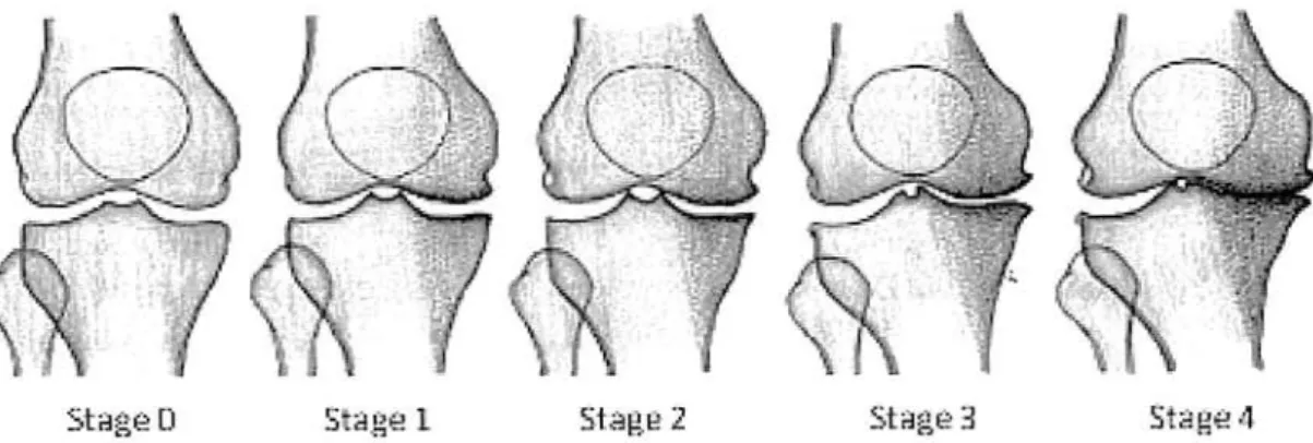
2.3.2 Kellgren-Lawrence Score

Diagnosis of knee osteoarthritis (OA) is typically performed though identification of bone changes and joint space narrowing on radiographs is using the

Kellgrene-Lawrence (KL) scoring system [6]. This indirect measure of cartilage disease is likely preferred due to its relatively low cost and minimal requirements in analysis time. However, the earliest changes in cartilage degeneration are alterations in the biochemistry of the extracellular matrix of the cartilage and are unlikely to be observed on radiographs [7]. Stage 0 indicates no radiographic findings of osteoarthritis, stage 1 minute osteophytes of doubtful clinical significance, stage 2 definite osteophytes with unimpaired joint space, stage 3 definite osteophytes with moderate joint space

narrowing and stage 4 definite osteophytes with severe joint space narrowing and

11

subchondral sclerosis (Fig . 2-6).

U

.,

.. \

,\

,..

,1 i

IStAgu: 2Star-le3 .S'..,--:12..P.1

Figure 2-6 Schematic illustration of Kellgren-Lawrence Score

(http://www.juntendo.ac jp/hospital/clinic/seikei/kanja02_b.html)

2.3.3 Outerbridge classification

The Outerbridge classification (Fig. 2-7) is a grading system for joint cartilage breakdown. The Outerbridge classification is an invasive diagnostic method using arthroscopy, and elastic evaluation by an indenter is also performed simultaneously.

12

Fig. 2-7 Schematic

2.3.4 Modifi

The Modified Outerbridgeclassificationisagradingsysteminarthroscopyforjoint cartilage injury usingMRIbasedontheOuterbridgeclassification.

In modified Outerbridgeclassification,Grade0indicatsintactcartilage, 1: chondral softening orblisteringwithanintactsurface,grade2:shallowsuperficial ulceration,fibrillation,orfissuringinvolvinglessthan50percentofthedepthofthe articular surface, grade3:deepulceration,fibrillation,fissuringorachondralflap

0. Normal

1. Swelling and Softening

2. A partial-thickness defect

3. Fissuring to subchondral bone

4. Exposed subchondral bone

hematic illustration of Outerbridge classification [3]

Outerbridge classification using MRI

dge classification is a grading system in arthroscopy for joint /MI based on the Outerbridge classification.

uterbridge classification, Grade 0 indicats intact cartilage, de r blistering with an intact surface, grade 2: shallow superficial

or fissuring involving less than 50 per cent of the depth of the 3: deep ulceration, fibrillation, fissuring or a chondral flap

13

involving 50 per cent or more of the depth of the articular cartilage without exposure of subchondral bone and grade: full-thickness chondral wear with exposure of subchondral bone [8].

2.3.5 Quantitative cartilage imaging using MRI

Various proton relaxation times can be quantitatively measured in the articular cartilage.

Recently, with three different MR techniques, measurements of longitudinal, transverse relaxation times and spin-lattice relaxation time in the rotating frame (Fig. 2-8), have been reported. T1 is always measured after intra venous administration of

gadolinium-diethylene triamine pentaacetic acid (Gd-DTPA). The delayed gadolinium enhanced magnetic resonance imaging (MRI) of cartilage (dGEMRIC) is obtained and demonstrates preferential accumulation of the negatively charged contrast agent in cartilage with decreased PG content that causes diminution of proton T1 compared with normal tissue. Transverse relaxation time (T2) is proportional to the distribution of cartilage water and is inversely proportional to the concentration of PG. Spin-lattice relaxation time in the rotating frame (T1 p) correlates to PG content in articular cartilage and it is more sensitive to the change of PG than T2 [9].

14

Fig. 2- 8 the quantitative image of the cartilage by relaxation time T2-mapping (a) and T 1 p-mapping (b) in a porcine model.

1`il

IC4

5t

15

Chapter 3 Microscopic water molecule motion in the cartilage obtained from diffusion weighted images

3.1 Free diffusion

Molecular diffusion refers to the random translational motion of molecules called Brownian motion, which results from the thermal energy carried by these molecules [1].The movement of molecules causes normal probability distribution, and the quantity of movement of molecules is proportional to concentration gradient macroscopically.

This proportional constant is diffusivity D which is based on a particular solution of the diffusion equations (1).

ac(x, t) _Da2c(x, t)

at-ax(1)

One of the special solutions of the diffusion equation shows normal distribution in point spread function (2).

1---

exp—x(2) / 42rDt 4Dt

Another special solution of the equation shows a sine wave in frequency response.

exp[ Dk2tjsinkx(3)

16

The distribution of magnetization made in a gradient magnetic field shows the solution of the diffusion equation. The signal intensity decays exponentially but the shape of the distribution with time is unchangeable, and the degree of the decay signal depends on diffusivity D and spatial frequency k. The diffusion weighted image uses bipolar gradient in Echo Planner Imaging (EPI) sequence (Fig. 3-1). Bipolar gradient i.e., motion probing gradient (MPG) causes dephasing of spins by the first gradient.

90° pulse180° pulse

MPG"

MPG

A

G: magnitude of the gradient, (3: time to apply of MPG (diffusion time), A: interval between MPG Fig. 3-1 Schematic representation of diffusion weighted image sequence

Stationary tissue is rephased at the end of the second opposite MPG; therefore,

stationary tissue reveals high signal intensity. In tissue with molecular movement of

17

water protons, a signal loss occurs since the protons have moved out by the time of the

rephasing opposite gradient. The greater the mean free path length of the water

molecules, the greater is the signal loss achieved with a diffusion-weighted sequence .

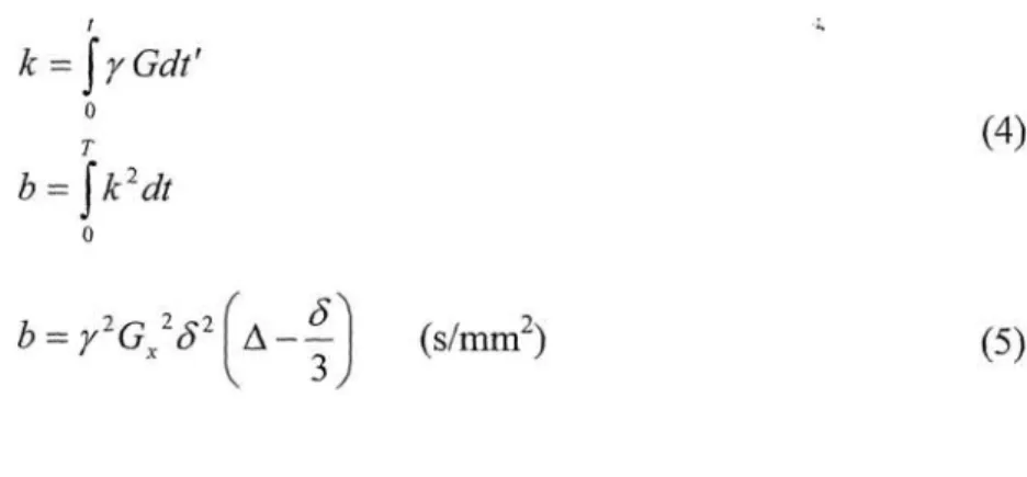
The strength of MPG is given with a b value in the following equation;

I ..-

k = f 7 Gdt1

T(4)

b = fic2 dt

0

I cY

b = 72G „2 (52 A --- (s/mm2)(5) 3

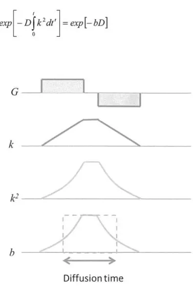
Figure 3-2 shows relations of k and b value in applying bipolar gradient . The diffusion

phenomenon applies to random movement (incoherent motion) of innumerable protons.

The diffusion weighted image is influenced by coherent motion and cannot distinguish coherent motion from incoherent motion in voxel. The strength of MPG is indicated by b value. Since strong MPG reduces the signal of the fast moving molecules

, application of high b value is suitable to assess slowly moving molecules . Amplitude of the b value has a trade-off relation with the signal intensity , as well as, defines the image contrast. From the special solution of the diffusion equation using sine wave , the change of the signal intensity is given in a following expression;

18

exp — D k2 dt ' = expt— bD1(6)

k2-

b ---

Diffusion time

Fig. 3-2 Schematic representation of G, k, b

3.2 Restricted diffusion

For example, the movement of molecules in vivo is limited by a cell membrane

(anisotropic diffusion) and does not move freely (Fig. 3-3).

19

Dl

\\)D2

obstacles

/

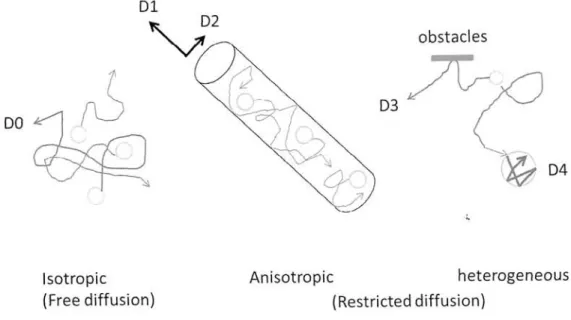
D3fz--7 DO

D4

IsotropicAnisotropicheterogeneous

(Free diffusion)(Restricted diffusion)

Fig. 3-3 Schematic representation of the interaction of diffusing molecules with various types of obstacles or constraints to free diffusing motion.

Isotropic diffusion is restricted as anisotropic or heterogeneous in human body (DO > D1 > D2, DO > D3 > D4).

Apparent diffusion coefficient (ADC) is distinguished from diffusivity D, since it represents the anisotropic diffusion of water molecules in vivo. ADC is calculated from two or more images obtained by different b values. The contrast in the ADC map depends on the spatial distribution of ADC and does not contain Ti and T2* values.

MRI can demonstrate the state of diffusion phenomenon in human body which is applied in a variety of clinical settings, especially in acute cerebral stroke at the

posterior part of the left middle cerebral arterial territory (Fig. 3-4).

20

Fig. 3-4 Diffusion weighted image of acute ischemic stroke

(Reference cited: Kumamoto general Hospital, http://www.cityhosp-kumamoto.jp/xsen/pg-MRI_00.html)

3.3 Diffusion in articular cartilage

Articular cartilage is a bi-phasic material: the permeable solid section which is represented by a solid matrix that consists of- collagen fibers and proteoglycan molecules, and the fluid section which is composed of extracellular water with dissolved ions and nutrients. Diffusion weighted imaging may offer information that is related to the integrity of the collagen network by investigating the nature of fluid dynamics in cartilage through its ability to distinguish between moving and stationary fluids [2]. Most of the fluid (Fig. 3-5) can move through the collagen network during loading. When the bound water restricted by a collagen network and proteoglycan is

21

subjected to loading, especially at weight bearing joints such as knee joints. When load is removed, the free water invades again, and the cartilage has the elasticity and the

property of viscosity by this action.

Bondage water

free water

unfreezable water cartilage

Fig. 3-5 Schema of fluid in articular cartilage model

As the way, the fluid dynamics in conjunction with the pore morphology and fluid transportation plays an important role in the overall mechanical function of the joint and ADC may become a new approach to diagnosis [3]. Macromolecules in the cartilage restrict the displacement of water compared with in bulk water; therefore the ADC is generally lower in cartilage than in bulk water. Burstein et al. reported

increases in ADC following enzymatic degradation of cartilage with trypsin, while

22

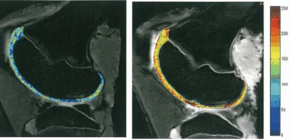
mechanical compression of the tissue resulted in a reduction in ADC [4]. Zhu et al.

reported both the DWI images and the ADC can provide insights into physiologic characteristics of patellar cartilage in vivo (Fig. 3-6). DWI reflects the microscopic of the tissue structure by water molecules that are undergoing random diffusion-driven movements. The collagen fiber of cartilage is anisotropic architecture [5], and the

self-diffusion of the water protons is characterized by a 3 x 3 tensor [6]. The Diffusion Tensor Imaging (DTI) can measure diffusion anisotropy of in vivo cartilage and the direction of the eigenvectors corresponding to maximum diffusion reflects the alignment of collagen fibers [7] (Fig. 3-7).

. „

(a)

.

.

/ • 1 k

t ,

"",.• •' A)., -

. .•

Fig. 3-6 Morphological image and ADC mapping of the knee.

Morphological T2star transverse image (a) and ADC-mapping of the knee (b). The ADC values were represented by different colors on the color maps of ADC; green areas were cartilage (b).

23

A

B

Fig. 3-7 DTI of human articular cartilage.

Baseline-preferred diffusion direction map (A). Preferred diffusion direction map for the same sample after treatment with trypsin and collagenase (B). Reference cited: Deng X et al. / MRI 2007.

24

Chapter 4 Evaluating relation between apparent diffusion coefficient and viscoelasticity of the cartilage

4.1 Introduction

In the early stages of OA, conservative treatment is often recommended to prevent the

progression of degenerative changes in articular cartilage. These changes include the disruption and/or alteration of the extracellular matrix, in such forms as decreased concentration of proteoglycans, increased water content, or deterioration of collagenous architecture, all of which have been demonstrated biologically and histologically [1-2] .The application of quantitative MR imaging techniques to degenerative cartilage has been a focus of recent research [3-4]. Quantitative MR imaging techniques, such as T2 relaxation time mapping [5-6], T 1 p relaxation time mapping [7-9], delayed gadolinium-diethylene-triamine-penta-acetic (Gd-DTPA) -enhanced MR imaging of cartilage (dGEMRIC) [ 10], and apparent diffusion coefficient (ADC) mapping [11], have been reported as useful indicators of degenerative changes in cartilage extracellular matrix, which consists of proteoglycans, collagen, non-collagenous proteins, and water. T2 measurements in cartilage have been

25

shown to correlate with collagenous architecture and water content [5], while T 1 p measurements in cartilage have been shown to correlate with proteoglycans and water content [12]. The dGEMRIC technique has been shown to correlate mainly with

proteoglycans. ADC measurements, on the other hand, have been shown to correlate mainly with water content and collagen matrix structure in cartilage. [13-14]. It has been shown that water and the collagen matrix produce the flow-dependent viscoelasticity of cartilage [15]. Thus, ADC can serve as an ideal indicator of the viscoelasticity of cartilage. Several studies have addressed the relationship between ADC and viscoelasticity. Juras et al. reported that ADC correlates with relaxation time in superficial zones using specimens in different stages of degeneration from patients who had undergone total knee replacement surgery [16]. Topographic variation in the cartilage matrix has also been shown to exist [17-19]: weight-bearing regions receive direct compression and tensile loading during walking, while non-weight-bearing regions receive less loading. Yet topographic variation in terms of ADC and viscoelasticity has not been previously studied. The aim of this study was to investigate correlation between ADC, Tlp and the viscoelasticity using porcine knee cartilage.

26

4.2 Theory supported Tip

4.2.1 Spin-Lock pulse

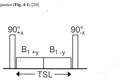
The initial nonselective 90° pulse along the +x axis nutates the magnetization into the transverse plane along the +y axis. The magnetization vector is then spin-locked with amplitude B1 for a duration of TSL with an on-resonance spin-lock pulse applied in line with the magnetization vector along the y axis. The spin-lock pulse is split into two

phase-alternating halves along the positive and negative y axes to reduce the effects of B1 inhomogeneity. At the end of the spin-lock pulse, the magnetization vector is nutated back into the longitudinal axis using a nonselective 90° pulse along the -x axis . This pulse cluster is preencoded before a read-out sequence to create a single-slice spin-lock pulse sequence (Fig. 4-1) [20].

a(),„900

+X -x

B1 ±y B1

4----TSL--- 0.

Fig. 4-1 Schematic of a Tip-weighted spin-lock RF pulse cluster

27

The equilibrium longitudinal magnetization MO is tilted to the transverse plane by a 90° RF pulse. This is followed immediately by a locking RF pulse BSL, which is applied during the locking time TSL. The phase of BSL is adjusted so that it is parallel aligned with the tilted magnetization vector M (Fig. 4-2) [21].

zT

Fig. 4-2

in

Magnetization vector M

homogeneous field Bloc .

()

during the SL

B , ..

pulse B

with amplitude BSL in an

4.2.2 Magnetization in the rotating frame

T 1 p pre-pulse sequence consists of a 90°y pulse to bring the magnetization along (for example) the x'-axis, followed by a long "lock" pulse, exiting a B1 field along the x'-axis. This lock pulse prevents T2 dephasing of spins. The spins are after some time

28

brought back in the longitudinal direction with a 90° "flip-up" pulse. During the locking pulse there is interaction of the free water proton spins with the spins of the macromolecules, causing T 1 p decay depending on the relative amount of macromolecules and their properties, somewhat similar to the processes governing magnetization transfer contrast (MTC). This prepulse was originally applied at very low fieldstrength, where the inhomogeneties of the main magnetic field are unimportant. At high fieldstrength with large absolute values of field inhomogeneities,

a composite Tlp prepulse yields better locking [22].

The magnetization (M) begins along the z-axis in the equilibrium position (a) and is nutated into the y-axis by the initial hard 90° along the x-axis. The magnetization then nutates in the rotating frame about the SL pulse applied along the y-axis (b). At the end of the spin-lock pulse duration (TSL), the magnetization is left in the transverse plane (c). The magnetization is then restored to the longitudinal axis by the second hard 90° applied along the negative x-axis (d). The resultant T 1 p-prepared magnetization is ready to be read using gradient echo (GRE) or spin echo (SE) readout.

Residual transverse magnetization is destroyed using a crusher gradient immediately following the second hard 90° pulse (Fig. 4-3) [20] .

29

Z ZZZZ

MI M

SL =>90-x

-~y->yyy

SL

/ 90+X

xxxMx x

abcde

Fig. 4-3 Vector diagram of the nutation of the magnetization in the rotating frame of reference.

T 1 p mapping is a quantitative MRI technique that has been used to evaluate degenerative changes in the extracellular matrix of cartilage [23]. Tlp can be measured through a combination of pulse sequences designed to obtain spin-lock pre-pulse and

contrast. T1 p sequences are typically combined with readout sequence such as three-dimensional (3D) GRE sequences [24-26] to decrease both the scan time and the specific absorption rate (SAR) [20, 24].

4.2.3 Tlp-prepared segmented multi-shot 3D-TFE sequence

The pulse sequence diagram is shown in Fig. 4-4. Initial longitudinal magnetization

(M0, t= 0), spin-lock RF pulse (SL-RF), post SL-RF longitudinal magnetization (MA, t = ta), longitudinal magnetization after n RF pulses (MB, t = tb), recovered longitudinal magnetization (MC), and post-SL-RF longitudinal magnetization (MD).

30

Recovery time (t) = shot interval- (TR x n+ TSL) > Ti x 5. Longitudinal magnetization changes from Mo to MA, MB, MC, and MD. Tip weighted signals were recorded during the transient state to avoid measurements during a steady state.

The signal intensity was measured when the k-space was filled from low to high (in centric order) immediately after the spin-lock signal (MD) fills k = 0. The time required to reach steady state depends on the Ti value of the tissue; in tissues with a short Ti, such as adipose tissue, steady state can be achieved immediately. In contrast, in tissues with a long Ti, such as water, the transient state continues until the end of the data collection period.

Recovery time T urbo factor: n

Shot-inten,a1 - (TR X TSL)

1 MI II SIN

C--->

• 1 _~r

SL-RF

SIMF

FT-1F-Al171-1EllImM171-113

Fig. 4-4 Schematic diagram of the common Tip prepared GRE sequence

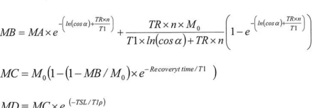
Changes in the longitudinal magnetization of each period are given by the following formulas:

31

(--TSL / Tip) MA = M O X e

/(

In(c o s cr)+TRxn`

hi(cos a)+TRxn` TR x n xM

oTi MB

= MA x eT1--- 1 — e

T1 x ln(cos a) + TR x n MC = M0(1— (1— MB / M 0)x e- Re covelyt time/Ti )

MD mc x e (-TSL / Tip)

where a is the flip angle and n is number of RF pulses (TFE factor).

4.2.4 Behavior of the magnetization of the transient period

The transient response (Fig. 4-5) is the magnetization during the initial period of a sequence during which steady-state magnetization M„ evolves from a particular initial condition. The length and character of the transient response depends on Tip, T2p, and the initial condition, Mo [27].

Fig. 4-5 Transient response of magnetization from Mo to Mss

32

The real-valued eigenvector, V„ is shown. The component of the transient response which is

directed along V, decays exponentially. The component that is orthogonal to V, decays along a

circular spiral path in the plane almost orthogonal to V,.

4.2.5 Artifact

If the magnetization vector is poorly aligned with the spin-locking pulse, there is ample opportunity for it to undergo pronounced off-axis nutation. This occurs in the case of an inhomogeneous B1, where nutation angles are spatially varying and may result in dramatically non-uniform image artifacts that markedly degrade any attempts at

quantitative imaging (Fig. 4-6).

FA10°FA30°FA50°

Fig. 4-6 Artifact of the phantom image depending on the FA

33

4.3 Basic points of mechanical property

4.3.1 Viscoelasticity

Viscosity is a measure of the resistance of a fluid which is being deformed by either shear stress or tensile stress. Water is a lower viscosity, while honey is a higher viscosity. The less viscous the fluid is, the greater its ease of movement (fluidity).

Young's modulus, also known as the tensile modulus or elastic modulus, is a measure of the stiffness of an elastic material and is a quantity used to characterize materials. It is defined as the ratio of the uniaxial stress over the uniaxial strain in the range of stress.

v, v, cv (r)

Strain E

Fig. 4-7 Stress-Strain Curve

34

Viscoelasticity is the property of materials that exhibit both viscous and elastic characteristics when undergoing deformation. Viscous materials, like honey, resist shear flow and strain linearly with time when a stress is applied. Elastic materials strain instantaneously when stretched and just as quickly return to their original state once the stress is removed. Viscoelastic materials have elements of both of these

properties and, as such, exhibit time-dependent strain.

4.3.2 Effect of temperature on viscoelastic behavior

Thermal motion is one factor contributing to the deformation of polymers, viscoelastic

properties change with increasing or decreasing temperature. An increase in

temperature correlates to a logarithmic decrease in the time required to impart equal

strain under a constant stress.

4.3.3 Stress relaxation

Stress relaxation describes how polymers relieve stress under constant strain. Because

they are viscoelastic, polymers behave in a nonlinear.

35

This nonlinearity is described by both stress relaxation and a phenomenon known as

creep, which describes how polymers strain under constant stress.

E E0---

0

-7-C 3 2

(4;1

toTime (s)

Fig. 4-8 Stress-Relaxation Curve

Figure 4-8 shows the response of a Standard Linear Solid material to a constant stress

ao, over time from to to a later time tf. For times greater than tf the load is removed.

The curvatures of the model represent the effects of both creep and stress relaxation.

36

4.4 Material and Methods

4.4.1 Subjects

Fresh porcine knee joints (n =20, age 6 months) were obtained from a local abattoir (ZEN-NOH Central Research Institute for Feed and Livestock, Ibaraki, Japan). Because we used branded edible pigs, which for quality-control purposes are slaughtered

precisely six months after birth, all pigs had almost finished growing but remained skeletally immature.

4.4.2 MR Imaging

MR imaging was performed within 30 hours after euthanasia. Specimens were kept at room temperature (20°C) for three hours before MR imaging. MR imaging was

performed on a 3.0-T whole-body clinical scanner (Intera Achieva; Philips Medical Systems, Best, Netherlands) with an 8-ch SENSE (sensitivity encoding) knee coil using a parallel imaging technique. Sagittal MR images were acquired along a plane

perpendicular to the line which passes though the medial femoral condyle and the lateral femoral condyle. In this plane, we did not evaluate the tibial and patellar cartilage to avoid any partial volume effect due to surrounding structures. Morphological isotropic

37

images were acquired using a three-dimensional fast field echo (3D-FFE) sequence, ADC of cartilage was measured using a single-shot spin echo-echo planar image sequence and three-dimensional Tip prepared turbo field echo (3D-TFE) sequence showed in Table 4-1, where repetition time: TR, echo time: TE, field of view: FOV, excitations: NEX, spin lock time: TSL, flip angle: FA.

Table 4-1 Scan parameters

TR/TE 1 /TE2 FOV Matrix (interpolated matrix)

Slicethickness/

gap/Number

NEX

TSL FA/

spin lock amplitude Total Acq.time

3D-FFE 19/7.0/13.3 MS

1 SO 256x 256 (512 x 512) 0.3mm/ 0/250 Isotropic voxel

35 degree

5'09-

ADC 4000/47 120x 120

12$ x128 (256 x 256) 3 mm/0. 3 mm! 19

0,700,1000.1500 shrim2

90 degree

Tlp 1?/9.?

120 256 x 236 3 nun/0 nun/ 19

1

L10.20.40.80 ms 10 degree/ 500 Hz

22L(eachTSL)

An ADC map was generated from diffusion weighted images using the built-in software that accompanies the clinical scanner (Philips). An ADC map was generated

38

on a pixel-by-pixel basis by fitting the b value data from the measured signal intensity

(Sb) attenuation according to a mono-exponential decay equation, as follows:

S(b) = S(b =O) exp (— bD)

A Tip map was generated on a pixel-by-pixel basis by fitting the TSL value data from the measured signal intensity (STSL) attenuation according to a mono-exponential decay

equation, as follows:

S(TSL) = S(TSL-o) exp(— TSL / T1 p)

4.4.3 ROI setting

Four sites in each specimen, namely, the medial femoral condyle, the lateral femoral condyle, the medial trochlea, and the lateral trochlea, were analyzed by means of both MR imaging and indentation testing (Fig. 4=9). For each specimen, a region of interest

(ROI) was drawn on the slice which passed through the center of the medial femoral condyle, the lateral femoral condyle, the medial trochlea, and the lateral trochlea. This ROI was drawn to include the weight-bearing area of the medial and lateral condyles and the non-weight-bearing area of the medial and lateral trochleae. Furthermore, the cartilage was divided along a line parallel to the cartilage/bone interface into two layers

(superficial and deep) of equal thickness. An ROI was drawn over the entire superficial

39

layer as it has been shown that degenerative changes begin in the superficial layer, and

also because mechanical testing mainly reflects the properties of the superficial layer of

cartilage. All ROIs were drawn manually by a single investigator.

(c)

Fig. 4-9 Image of the ROI

MR image of weight-bearing region (a) and non-weight-bearing region (b), Indenter testing points of weight-bearing region (c) and non-weight-bearing region (d)

40

4.4.4 Mechanical testing

Indentation testing (Fig. 4-10) was performed on an electromechanical precision controlled system (Vesmeter E-200DT; WaveCyber Co., Ltd., Saitama, Japan). The shape of the indenter tip is a cone with an angle of 30 degrees, a tip diameter of 0.1 mm, and a pressurization of 35 grams each 0.2 second. Measuring one region takes less than 2 minutes.

.11'~1r!

5

Fig. 4-10 Image of the indenter test device

Indentation testing device (a) and the appearance under measurement of porcine knee cartilage in situ (b). A shape of the tip of the indenter is cone of 30 degrees, tip diameter of 0.1 mm, and pressurization of 35 gram.

41

This device can provide the viscosity, elasticity, relaxation time, elastic rate, stiffness,

and strain depth as given by Voigt's equation:

S=Gy+77• dy dt

where y denotes displacement, G is elastic modulus, denotes viscosity and S is stress.

Indentation testing was performed on the same regions that were selected for MRI

analysis. Two lines consisting of five points per line at intervals of 3 - 4 mm were tested

for a total of 10 points in each region. Viscosity coefficient and relaxation time were

measured as indicators of the viscoelasticity of cartilage. To minimize the possibility of

measurement errors during indentation tests, the mean viscosity coefficient and

relaxation time obtained for all ten points in each region were taken as the viscosity

coefficient and relaxation time for that region. During mechanical testing, the specimens

were wrapped in moist gauze to prevent them from drying.

4.4.5 Statistical analysis

The relationship between ADC and viscosity coefficient as well as that between ADC

and relaxation time were assessed by means of correlation analysis. The correlation

coefficients were assessed using a Pearson coefficient. Significant differences among

the weight-bearing, non-weight-bearing, medial, and lateral regions were evaluated by

42

multiple comparison tests using one-way analysis of variance (ANOVA). Statistical significance was defined as p<0.05. Statistical software (Statcel for Windows, OMS, Saitama, Japan) was used for all analyses.

4.5 Results

All porcine knees were visually healthy, with no blistering, ulceration, fissuring, or thinning of cartilage. ADC was correlated with relaxation time and viscosity coefficient

(R2=0.75 and 0.69, respectively, p<0.01) (Fig. 4-11, 4-12).

• FT (wb) > PF (nwb)

1600

1400^

E E 0 x V

1200

1000

800

600

400

200

0

a^ ®^

^ Et

no a I al

talt , E

sal rszi

R2 = 0.75, p.<0.01 200

0

00.20.40.60.81

relaxation time (ms)

Fig. 4-11 Correlation between ADC and relaxation time

A significant correlation between ADC and relaxation time was observed. The ADC of the weight-bearing region was significantly higher than that of the non-weight-bearing region.

43

^FT(vvb) 1600 ---'-

1400 r---^-- 1200 ^--- 1000 ---

800 ^^--- 600 ^---^--- 400 ^--- 200 ^'---

0

0 1000

PF(nvvb)

E 0

^^^^^^^^^

-- ^

^^^

.~.

• ^

m

R2 = 0.69 p<0.01

2000 3000 4000 5000 viscosity cofficient (kPa • s)

6000 7000

Fig. 4-12 Correlation between ADC and viscosity coefficient

A significant correlation between ADC and viscosity coefficient was observed. The ADC and the viscosity coefficient in the weight bearing region were significantly higher than those in the

non-weight bearing region.

On the other hand, Tip was poorly correlated with relaxation time and viscosity coefficient (R2=0.17 and 0.26, respectively, p<0.01) (Fig. 4-13). The mean relaxation time values in the weight-bearing and non-weight-bearing regions were 0.61+0.17 ms and 0.14+0.08 ms, respectively (Table 4-2). The mean viscosity coefficient values in weight-bearing and non-weight-bearing regions were 5043+787 kPa • s and 3100±806 kPa • s , respectively (Table 4-2).

44

350.00 300.00 250.00 200.00 150.00 100.00 50.00 0.00

Fig.

• FT (wb)

•C PF (nwb)

0 0•

0• •••

•• 0

to • 44 • (9)(D& 0 0•40 • • 4,....•,_

4..••IP orb 4fr

• *•

Att:•°0'°••IF.

•

voi-r,00••V%I0I. _'114'0 :

to) 0

0•

o

R2 = 0.17 p<0.01

00.20.40.60.81

relaxation time (ms)

4-13 Correlation between Tip and relaxation time

Table 4-2 ADC, Tip and mechanical property of cartilage *p<0 .05

FT PF

ADC (mm2 /s) Tip (ms)

viscosity coefficient

(N•s/m2) Relaxation time (ms,)

1088 125*

182.97 ±-35.71*

5.04 ± 0.79*

0.61 ± 0.17*

835 ± 110*

168.01 ±24.29*

3.10 ± 0.81*

0.14± 0.08*

45

Weight-bearing regions had significantly longer relaxation times and higher viscosity coefficient values than non-weight-bearing regions did (p<0.05). The mean ADC values in weight-bearing and non-weight-bearing regions were 1087+125x10-6 mm2/s and 835+110x10-6 mm2/s, respectively (Table 4-2). The mean Tip values in weight-bearing and non-weight-bearing regions were 182.97±35.21 ms and '-168.01±24.29 ms, respectively (Table 4-2). All of these differences were statistically significant (p<0.05).

4.6 Discussion

Cartilage plays a critical role in joint function, where it acts as a shock absorber during

joint loading. This function is partly enabled by proteoglycan, which has a high negative charge and binds to water molecules, thereby generating the swelling pressure of cartilage [28]. This swelling pressure is counteracted by the tensile strength of cartilage, which is provided by a dense and regularly arranged collagen network

[29-32]. Therefore, intermolecular interactions of both major components of cartilage with water molecules give cartilage its viscoelasticity, the characteristic that enables cartilage to act as a shock-absorber [15, 33]. The decrease in proteoglycans and disruption of the collagen network that occurs over time in degenerative cartilage leads

46

to a loss of viscoelasticity [16].

It has been suggested that differences in diffusivity as assessed by ADC may be due to differences in water mobility, which in turn is determined by the average

pore size in the cartilage matrix [34-35]. The difference in diffusivity between tibiofemoral and patellofemoral cartilage, for example, might be due to differences in their inherent matrix structures and compositions. Indentation testing can directly evaluate the viscoelasticity of cartilage, and has been used in several studies to assess cartilage function in degenerative cartilage [36]. Recent studies have used arthroscopic indentation instruments for this purpose, but such indentation testing is somewhat invasive and should not be used as a routine clinical evaluation method. In comparison, MR imaging is less invasive and can be used more regularly for clinical evaluation.

This study has uncovered significant correlations between ADC and relaxation time, as well as between ADC and viscosity coefficient, indicating that ADC can serve as an ideal measure of cartilage viscoelasticity.

There are several limitations of this study. First, only visually healthy cartilage specimens were recruited. Thus the usefulness of ADC as a means of assessing degenerative cartilage remains unknown. In addition, as biochemical and histological

analysis were not performed, the usefulness of ADC as a quantitative measure of

47

cartilage degeneration is also unknown. These deficiencies constitute major weaknesses of this study.

As cartilage samples from several different regions of several different

porcine knees were used, specimens with various cartilage matrix compositions were included. Therefore, the significant correlation observed between ADC and viscoelasticity lends support to the notion that ADC could be useful in the evaluation of degenerative cartilage as well. Further studies including knees with degenerative cartilage and incorporating biochemical and histological analysis are needed to confirm this. At present, however, it is unknown whether the results of the current study may be

applied to the evaluation of repaired cartilage, degenerating cartilage, and/or mature knees.

A second limitation is that the indentation test was the only mechanical test

performed on our cartilage samples. It has been shown that cartilage exhibits a much greater stiffness in tension than in compression, and that cartilage exhibits anisotropy in tension and compression. Further studies using other mechanical tests including tension tests may reveal a more detailed relationship between ADC and data on cartilage strength.

Third, we did not use any models of defective or degenerating cartilage in this

48

study, as we used only tissues from branded edible pigs, and as only immature porcine

knees were included. It will be necessary to determine whether similar results can be

obtained using repaired cartilage, degenerating cartilage, and/or mature knee cartilage

in future studies before ADC is used clinically as a measure of cartilage viscoelasticity.

4.7 Conclusion

A moderate correlation was observed between ADC and viscoelasticity in superficial

articular cartilage. Both molecular diffusion and viscoelasticity were higher in

weight-bearing than in non-weight-bearing regions of articular cartilage.

49

Chapter 5 Evaluating relation between speed of sound and elasticity of the cartilage

5.1 Introduction

In previous studies, degeneration of cartilage was trying to be assessed by high frequency ultrasound by paying attention to the thickness, morphology, and surface roughness of cartilage [ 1-8], however, these tools cannot be used in vivo. In contrast, the pulse-echo method provides high-resolution images of articular and periarticular structures by real-time imaging display. The imaging assessment of the cartilage has been improved by the advent of the pulse-echo method with a wide dynamic range [9].

Evaluation of changes in the thickness and elasticity of cartilage is important for assessing its degeneration. Further, some studies have compared the measurement results of cartilage thickness using ultrasound with those obtained using optics, needles, microscopes in vitro [7-8].

In addition to morphology, conventional ultrasound elastography based on speckle tracking has been used as a noninvasive method for evaluating elasticity in several types of tissue, however, its application in cartilage is difficult, since cartilage

50

itself does not have any echo signals [10-11]. As an alternative, when the cartilage is assumed to be a solid with isotropic linear elasticity, the relationship among the SOS

(c), density (p) Young's modulus (E), and Poisson's ratio (v) is expressed as follows:

c = VE(1—v)/p(1+vX1-2v)(1)

Therefore, the elasticity of cartilage can be assumed by the SOS in it which is calculated from the thickness of a given cartilage and the propagation time of the ultrasound within it [8, 12]

In this study, the accuracy of our proposing method of combination of MRI and ultrasound via the pulse-echo methods (combination method) in the assessment of SOS of cartilage that should correlate with the severity of its degeneration is evaluated. In the imaging of the cartilage by the pulse-echo method, longitudinal wave of the ultrasound was used. In the current study, preciseness of MR measurement of objects' thicknesses and accuracy of SOS provided by the combined method were first evaluated in agar phantom followed by in porcine knee cartilage. The applicability of the combined method to humans was also examined.

51

5.2 Theory supporting the speed of sound measurements

5.2.1 Basic ultrasound

Ultrasound is simply sound waves, and some physical properties are dependent on the frequency. Sound consists of waves of compression and decompression of the transmitting medium (e.g. air or water), traveling at a fixed velocity. Sound is an example of a longitudinal wave oscillating back and forth in the direction the sound wave travels, thus consisting of successive zones of compression and rarefaction.

Transverse waves are oscillations in the transverse direction of the propagation (Fig.

5-1).

ultrasonic longitudinal wave

densenon-dense

a_

time

Fig.

wavelength A

Spread direction of the sound wave

Cycle: T(s)f= 1 IT

wavelength : 2 (in) Frequency f (1/s)

Spped of sound : c (m/s)

5-1 Longitudinal compression wave and transverse wave

52

Basically, all ultrasound imaging is performed by emitting a pulse, which is partly reflected from a boundary between two tissue structures, and partially transmitted (Fig.

5-2). The reflection depends on the difference in impedance of the two tissues. Basic imaging by ultrasound does only use the amplitude information in the reflected signal.

One pulse is emitted, the reflected signal, however, is sampled more or less continuously (actually multiple times). As the velocity of sound in tissue is fairly constant, the time between the emission of a pulse and the reception of a reflected signal is dependent on the distance; i.e. the depth of the reflecting structure. The reflected pulses are thus sampled at multiple time intervals (multiple range gating), corresponding to multiple depths, and displayed in the image as depth (Fig. 5-2).

rReflectio

Medium 1

-

Medium 2

R=(Z)-ZI)// (Z 1±Z))

TransmissionT=1-R=2Z1 /(Z1+Z-3

Fig. 5-2 Reflection and transmission

53

The amplitude of the reflected signal, is not only dependent on the reflection

coefficient. The direction of the reflected signal is also important.

- An irregular scatterer will reflect only a portion back to the probe .

- A more regular scatterer will reflect more if the reflecting surfaces are

perpendicular to the ultrasound beam.

A

II

Fig. 5-3 Scatter and reflecting surfaces

5.2.2 Incidence angle and the distance

In a thickness measurement, the distance when a beam was incident perpendicularly

becomes the minimum. Oblique incidence causes artifacts by scatter.

54

dl

..----...--b-giVc

Fig. 5-4 Incidence angle and the distance

Perpendicularly incident (a), oblique-incidence (b), distance (c).

5.2.3 The transmission method measurement of speed of sound (SOS)

The transmission method was implemented using planar non-focusing transducers with a center frequency of 5 MHz and an aperture diameter of 0.25 inch (124-340, GE Inspection Technologies, Wichita, KS, USA) by noncontact at a distance of 30 mm.

Each agar phantom was placed in a laboratory dish filled with saline with through-transmission geometry, and the propagation time was measured without and with the agar phantom at room temperature (18.4°C) (Fig. 5-5a, b). Measuring and averaging the time between multiple echoes yields highly precise propagation times

(Fig. 5-5c).

SOS was measured according to the following formulae, where /I is the

distance between the transducer and the agar phantom, 12 is the specimen thickness, co

55