範囲基準下の最適停止について (不確実性と意思決定数理の諸問題)

範囲基準下の最適停止について

長崎大学経済学部 津留崎和義(Kazuyoshi Tsurusaki)

FacultyofEconomics, Nagasaki Univ.

九州大学大学院経済学研究院 岩本誠一 (Seiichi Iwamoto)

Graduate School ofEconomics, Kyushu Univ.

1

Introduction

Inthispaper, weconsider the optimal stopping problem for compoudcriteria, whose counterpart

is simple criteria such

as

terminal, additive and minimum. We introduce

a new

notion of gain

process, which is evaluated at stopped state. Some of gain processes

are

terminal, additive,

minimum, range, ratio, sample variance. The former three are simple. The latter three are

compound. In this paper

we

discuss the compond criterion such

as

range, mid-range, ratio,

average and sample variance.

2

General Process

We consider

a

class of finite-stage optimal stopping problems from

a

view point of reward

accumulation. An $N$-stageproblemhas to stop bytime$N$ at the latest. Each stage allowseiher

stop orcontinue. When adecision maker stops on astate at $n$-th stage, she gets arewardwhich

is closely related to all the states she has experienced.

Let $\{X_{n}\}_{0}^{N}$ be

a

Markov chain on

a

finite state space $X$ with

a

transition law $p=\{p(\cdot|\cdot)\}$

.

Letting $X^{k}:=X\cross X\cross\cdots\cross X$($k$ times) be the direct product of $k$ state spaces $X$,

we

take

$H_{n}:=X^{n+1}$; the set of all subpaths $h_{n}=x_{0}x_{1}\cdots x_{n}$ up to stage $n$ :

$H_{n}=\{h_{n}=x_{0}x_{1}\cdots x_{n}|x_{m}\in X, 0\leq m\leq n\}$ $0\leq n\leq N.$

In particular,

we

set

$\Omega:=H_{N}$.

Its element $\omega$ $=h_{N}=x_{0}x_{1}\cdots x_{N}$ is called

a

path.

Let$T_{m}^{\iota}$ be the set of all subsets in $\Omega$which

are

determinedbyrandom variables $\{X_{m},X_{m+1}$,

,

.

.,$X\mathrm{J}$ where $X_{k}$ : $\mathit{1}arrow X$ is the projection, Xk(u) _{$=x_{k}$}. Strictly, $\Psi_{m}^{\iota}$ is the $\mathrm{c}\mathrm{r}$-field

on 0

generated by the set ofall subsets ofthe form

$\{X_{m}=x_{m}, X_{m+1}=x_{m+1}, \ldots, X_{n}=x_{n}\}(\subset\Omega)$

where $x_{m}$,$x_{m+1}$,. ..,$x_{n}$

are

all elements in state space $X$. Let

us

take $\mathrm{N}=\{0, 1, \ldots, N\}$. A

mapping$\tau$ : $El$ $arrow$ $\mathrm{N}$ is called

a

stopping timeif

$\{\tau=n\}\in\Psi_{0}$ $in\in$ N.

where $\{\tau=n\}=$ $\{x_{0}x_{1} . . . x_{N}| \tau(\mathrm{t}_{0}x_{1} . . . x_{N})=n\}$. The stopping time $\mathrm{r}$ is called $\{f_{0}\}_{0}^{N_{-}}$

adapted. Let $\mathcal{T}_{0}^{N}$ bethe set of all such stopping times. Any stopping time $\mathrm{r}$ $\in \mathcal{T}_{0}^{N}$ generates a

stopped subhistory (random variable) (Xo,$X_{1}$,

$\ldots$ , $\mathrm{X}$ 1,

$X_{\tau}$) on $\Omega$ through

Let $\{g_{n}\}_{0}^{N}$ be a sequence ofgain

functions

$g_{n}$ : $H_{n}arrow R^{1}$ $0\leq n\leq N.$

Then a gain process $\{G_{n}\}_{0}^{N}$ is defined by

$G_{n}:=g_{n}(X_{0}, X_{1}, \ldots, X_{n})$

.

Then any stopping time $\tau$ yields

a

stoppedreward (random variable) $G_{\tau}:)arrow 7$? :

$G_{\tau}(\omega)=G_{\tau(\omega)}(X_{0}(\omega), X_{1}(\omega),$ $\ldots,X_{\tau-1}(\omega)$,$X_{\tau}(\omega))$

.

Weremark that the expected value $E_{x_{0}}[G_{\tau}]$ is expressed by

sum

ofmultiple

sums

:

Then a gain process $\{G_{n}\}_{0}^{N}$ is defined by

$G_{n}:=g_{n}(X_{0}, X_{1}, \ldots, X_{n})$

.

Then any stopping time $\tau$ yields

a

stoppedreward (random variable) $G_{\tau}$ :

$\Omegaarrow R^{1}$ :

$G_{\tau}(\omega)=G_{\tau(\omega)}(X_{0}(\omega), X_{1}(\omega),$$\ldots$,$X_{\tau-1}(\omega)$,$X_{\tau}(\omega))$

.

Weremark that the expected value $E_{x_{0}}[G_{\tau}]$ is expressed by

sum

ofmultiple

sums

:

$E_{x0}[G_{\tau}]$ $=$ $\sum_{n=0}^{N}\sum_{\{\tau=n\}}G_{n}(h_{n})P_{x_{0}}(X_{0}=x_{0}, \ldots,X_{n}=x_{n})$

$N$

$=$

5

$\sum G_{n}(h_{n})p(x_{1}|x_{0})p(x_{2}|x_{1})$

.

.

.

$p(x_{n}|x_{n-1})$

.

$n=0\{\tau=n\}$

Now

we

consider the optimal stopping problem for the gainprocess :

Go(zo) ${\rm Max} E_{x_{0}}$$[G_{\tau}]$ $\mathrm{s}.\mathrm{t}$

.

$\tau\in$ $\mathcal{T}$$0N$

(

. (1)

Then

we

have the corresponding recursive equation and optimal stopping time ([4]) :

Theorem 2.1

$v_{N}(h)=g_{N}(h)$ $h\in H_{N}$

$Vn(h)={\rm Max}[g_{n}(h), E_{x}[v_{n+1}(h, X_{n+1})]]$ (2)

$h=$ $(x_{0}, \ldots, x_{n-1}, x)\in H_{n}$, $0\leq n\leq N-1.$

Theorem 2.2 The stopping time $\tau^{*}$ :

Vn(h) $= \min\{n\geq 0 : v_{n}(h_{n})=G_{n}(h_{n})\}$ $\omega$ $=$ xoxi $\cdot$$\cdot$

.

$x_{N}$

is optimal :

$E_{x_{0}}[G_{\tau}*]\geq E_{x0}[G_{\tau}]$ $\forall\tau\in \mathcal{T}_{0}^{N}$

3

Expanded

Control

Chain

Now, inthis section, letusdiscussageneral result forrange

process.

Weconsideramaximization

problem of expected value for stopped process under range criterion (As for nonstopping but

control problems,

see

[11-16, 21]$)$

.

Let $\{X_{n}\}_{0}^{N}$ be the Markov chain

on

the finite state space $X$ with the transition law $p=$ $\{p(\cdot|\cdot)\}$ (Section 2). Let $g_{n}$ : $Xarrow$p

$R^{1}$ b$\mathrm{e}$ a stop reward for $0\leq n\leq N$ and $r_{n}$ : $Xarrow R^{1}$ be

a

continue reward for $0\leq n\leq N-1.$ Then

an

accumulation process is constructed

as

follows.

When

a

decision-maker stops at stage $x_{n}$ onstage $n$ through asubhistory $(x_{0}, x_{1}, \ldots, x_{n-1})$, he

or she will incur the range ofreward up to stage $n$ :

where

$h_{n}=(x_{0}, x_{1}, \ldots, x_{n})$, $r_{m}=r_{m}(x_{m})$, $g_{n}=g_{n}(x_{n})$.

The accumulationprocess $\{R_{an}\}_{0}^{N}$is called

a

rangeprocess. Thus astopped reward by adopting

stoppingtime $\mathrm{r}$ for range process is

$R_{a\tau}=r_{0}\vee r_{1}\vee\cdots\vee r_{\tau-1}\vee g_{\tau}-r_{0}\Lambda r_{1}\Lambda\cdots\vee r_{\tau-1}\Lambda g_{\tau}$.

Now

we

consider the optimal stopping problem for range process :

Rao$(\mathrm{x}\mathrm{O})$ _{${\rm Max} E_{x_{0}}$} $[$ ? $\tau$

$]$ $\mathrm{s}.\mathrm{t}$. $\tau\in J\mathit{0}N.$

The expected value of range is the sum ofmultiple

sums

:

$N$

$E_{x_{0}}[h_{\tau}]=$ $\mathrm{p}$ $\sum\{R_{n}(h_{n})\mathrm{x}p(x_{1}|x_{0})p(x_{2}|x_{1}). . .p(x_{n}|x_{n-1})\}$ . $n=0\{\tau=n\}$

Let

us now

imbed $\mathrm{R}\mathrm{a}_{0}(x\mathrm{o})$ into a

new

class of additional parametric subproblems $[2, 17]$.

First

we

define the past-valued (cumulative) random variables $\{\tilde{\Lambda}_{n}\}_{0}^{N}$, $\{_{-n}^{-}-\}_{0}^{N}\sim$ up to _$n$-th stage

and the past-value sets $\{\Lambda_{n}\}_{0}^{N}$, $\{_{-n}^{-}-\}_{0}^{N}$ theytake :

$\mathrm{R}\mathrm{a}_{0}(x_{0})$ ${\rm Max} E_{x0}[R_{a\tau}]$ $\mathrm{s}.\mathrm{t}$. $\tau\in \mathcal{T}_{0}^{N}$.

The expected value of range is the sum ofmultiple

sums

:

$E_{x_{0}}[h_{\tau}]$ $= \sum_{n=0}^{N}\sum_{\{\tau=n\}}\{R_{n}(h_{n})\mathrm{x}p(x_{1}|x_{0})p(x_{2}|x_{1})\cdots p(x_{n}|x_{n-1})\}$.

Let

us now

imbed $\mathrm{R}\mathrm{a}\mathrm{o}(x\mathrm{o})$ into a

new

class of additional parametric subproblems $[2, 17]$.

First

we

define the past-valued (cumulative) random variables $\{\tilde{\Lambda}_{n}\}_{0}^{N}$, $\{_{-n}^{-}-\}_{0}^{N}\sim$ up to _$n$-th stage

and the past-value sets $\{\Lambda_{n}\}_{0}^{N}$, $\{_{-n}^{-}-\}_{0}^{N}$ theytake :

$\overline{\Lambda}_{0}:=\overline{\lambda}_{0}$ where $\overline{\lambda}_{0}$ is smaller than or equal to _{$g_{n}(x)$},$r_{n}(x)$

$–0=:=\tilde{\xi}_{0}$ where $\tilde{\xi}_{0}$ is larger than or equalto$g_{n}(x),r_{n}(x)$ $\overline{\Lambda}_{n}:=r_{0}(X_{0})\vee\cdots\vee r_{n-1}(X_{n-1})$

$–n=:=r_{0}(X_{0})\Lambda\cdots\Lambda r_{n-1}(X_{n-1})$

$\Gamma_{0}:=\{(\lambda_{0}, \xi_{0})\}$

$\Gamma_{n}:=\{(\lambda_{n}, \xi_{n})|$ $\xi_{n}=r0(x\mathrm{o})\bigwedge_{-}\cdots\Lambda r_{n-1}(x_{n-1})\lambda_{n}=r0(x_{0})\mathrm{v}_{1}\cdots\vee r_{n-1}(x_{n-1})(x_{0}, \ldots,x_{n})\in X\mathrm{x}\cdots \mathrm{x}X$

” $\}$ .

We have

Lemma 3.1 (Forward recursive formulae)

$\Lambda_{0}=\lambda_{0}$

$\tilde{\Lambda}_{n+1}=\tilde{\Lambda}_{n}\vee r_{n}(X_{n})$ $0\leq n\leq N-1$,

$–0==\tilde{\xi}_{0}$

$–n+1-\sim=--\sim-_{n}\Lambda r_{n}(X_{n})$ $0\leq n\leq N-1$,

$\Gamma_{0}=\{(\tilde{\lambda}_{0},\tilde{\xi}_{0})\}$

$\Gamma_{n+1}=\{(\lambda\vee r_{n}(x), \xi\Lambda r_{n}(x))|(\lambda, \xi)\in\Gamma_{n}, x\in X\}$ $0\leq n\leq N-1$.

Let us now expand theoriginal state space $X$ to adirect product space :

$\mathrm{Y}_{n}:=X\mathrm{x}$ $\Gamma_{n}$ $0\leq n\leq N.$

We define a sequence of stop-reward

_functions

$\{G_{n}\}_{0}^{N}$ by

$G_{n}(x;\lambda,\xi):=\lambda\vee g_{n}(x)-4$$\Lambda g_{n}(x)$ $(x;\lambda, \xi)\in t_{n}$’

We define a sequence of stop-reward

_functions

$\{G_{n}\}_{0}^{N}$ by

and

a

nonstationary Markov transition laut$q=\{q_{n}\}_{0}^{N-1}$ by

$q_{n}(y;\mu, \nu|x;)$ ,$\xi)$ $:=\{$

$p(y|x)$ if A $\vee gn(x)=\mu$, $\xi\Lambda vn\{v)=\nu$

0otherwise.

Let

us

define $\Gamma_{n}$ through

$\tilde{\Gamma}_{n}:=(\overline{\Lambda}_{n},\underline{-_{n}=})$.

Then $\{(X_{n}, \Gamma_{n})\}_{0}^{N}$ is

a

Markov chain

on

state spaces $\{\mathrm{Y}_{n}\}$ with transition law _$q$

.

We consider

the terminal criterion $\{G_{n}\}_{0}^{N}$ onthe expanded process :

$\overline{\mathrm{T}}$

o(yo) ${\rm Max} \mathrm{E}_{y0}[G_{\tau}]$ $\mathrm{s}.\mathrm{t}$. _$\tau\in$ $\mathrm{r}\mathrm{o}$

where $\mathit{1}0=$ ($x0;\tilde{\lambda}0$,$\tilde{\mu}$o), and

$\tilde{\mathcal{T}}_{n}^{N}$ is the set of all stopping times which take values in _$\{n$,$n\mathit{1}$

$1$,

. .

,$N$

}

on the

new

Markov chain.

Now

we

conside

a

subprocess whichstarts at state $y_{n}=(x_{n}; \lambda_{n}, \xi_{n})(\in \mathrm{Y}_{n})$

on

$n$-th stage :

$\overline{\mathrm{T}}_{n}(y_{n})$ ${\rm Max} \mathrm{E}_{y_{n}}[G_{\tau}]$ $\mathrm{s}.\mathrm{t}$.

$\tau\in\tilde{\mathcal{T}}$

:.

Let $vn(yn)$ be the maximum value of$\overline{\mathrm{T}}_{n}(y_{n})$, where

$v_{N}(y_{N})=G_{N}(y_{N})\triangle$ $y_{N}\in \mathrm{Y}_{N}$.

Then

we

have the the backward recursive equation :

Corollary 3.1

$\{$

$v_{N}(y)=G_{N}(y)$ $y\in \mathrm{Y}_{N}$

$vn\{v)={\rm Max}[G_{n}(y), \mathrm{E}_{y}[v_{n+1}(\mathrm{Y}_{n+1})]]$ $y$ $\in \mathrm{Y}_{n}$, $0\leq n\leq N-1$

where $\mathrm{E}_{y}$ is the one-step expectation operator induced

from

the Markov transition probabilities

$q_{n}(\cdot|\cdot)$ :

$\mathrm{E}_{y}[h(\mathrm{Y}_{n+1})]=\sum_{z\in Y_{n+1}}h(y)q_{n}(z|y)$.

Corollary 3.2 The stopping time $\tau^{*}$ :

$\mathrm{v}\mathrm{n}\{\mathrm{v}$) $= \min\{n\geq 0$ : $vn(yn)=Gn\{yn)\}$ $\omega$ _{$=y_{0}y_{1}\cdots$}

.

$y_{N}$

is optimal :

$\mathrm{E}_{y0}[G_{\tau^{\mathrm{r}}}]$ $\geq \mathrm{E}_{y0}[G_{\tau}]$ $\forall\tau\in$ $\mathrm{j}\mathrm{g}$ .

Then

we

have the corresponding recursive equation for the original process with maximum

reward :

where $y0=$ (#o;$\tilde{\lambda}_{0},\tilde{\mu}0$), and $\mathcal{T}\sim_{N,n}$ is the set of all stopping times which take values in $\{n,n+$

$1_{;}\ldots$,$N$

}

on the

new

Markov chain.

Now

we

conside

a

subprocess whichstarts at state $y_{n}=(x_{n};\lambda_{n}, \xi_{n})(\in \mathrm{Y}_{n})$

on

$n$-th stage :

$\overline{\mathrm{T}}_{n}(y_{n})$ ${\rm Max} \mathrm{E}_{y_{n}}[G_{\tau}]$ $\mathrm{s}.\mathrm{t}$. $\tau\in\tilde{\mathcal{T}}_{n}^{N}$.

Let $v_{n}(y_{n})$ be the maximum value of$\overline{\mathrm{T}}_{n}(y_{n})$, where

$v_{N}(y_{N})-=G_{N}(y_{N})$ $y_{N}\in \mathrm{Y}_{N}$.

Then

we

have the the backward recursive equation :

Corollary 3.1

$)$ $y\in \mathrm{Y}_{N}$

$G_{n}(y)$, $\mathrm{E}_{y}[v_{n+1}(\mathrm{Y}_{n+1})]]$ $y\in \mathrm{Y}_{n}$,

where $\mathrm{E}_{y}$ is the one-step expectation opemtor induced

from

the Markov transition probabilities

$q_{n}(\cdot|\cdot)$ :

$\mathrm{E}_{y}[h(\mathrm{Y}_{n+1})]=\sum_{z\in Y_{n+1}}h(y)q_{n}(z|y)$.

Corollary 3.2 The stopping time $\tau^{*}$ :

$\tau^{*}(\omega)=\min\{n\geq 0 : v_{n}(y_{n})=G_{n}(y_{n})\}$ $\omega$ _{$=y_{0}y_{1}\cdots\cdot y_{N}$}

is optimal :

$\mathrm{E}_{y0}[G_{\tau^{\mathrm{r}}}]\geq \mathrm{E}_{y0}[G_{\tau}]$ $\forall\tau\in\tilde{\mathcal{T}}_{0}^{N}$

Then

we

have the corresponding recursive equation for the original process with maximum

reward :

Theorem 3.1

$\{$

$v_{N}(x;\lambda, \xi)=\lambda\vee g_{N}(x)-\xi\Lambda g_{N}(x)$ $x\in X,$ $(\lambda, \xi)\in\Gamma_{N}$

$v_{n}(x;\lambda,\xi)={\rm Max}$

[

$\lambda\vee g_{n}(x)-\xi\Lambda g_{n}(x),$$E_{x}[v_{n+1}(X_{n+1;}$A$\vee r_{n}(x),$ $\xi\Lambda r_{n}(x))]$

]

(3)

Here

we

considerafamilyof subprocesses which start at $x_{n}(\in X)$ with

a

pairofaccumulated

maximum and maximum up to there $(\lambda_{n}, \xi_{n})$ :

${\rm Max} E_{x_{n}}$$[\lambda n\Lambda r_{n}\vee\cdots\vee r_{\tau-1}\vee g_{\mathcal{T}}-\xi_{n}\Lambda r_{n}\Lambda. ..\Lambda r_{\tau-1} \Lambda g_{\tau}]$

$\mathrm{R}\mathrm{a}_{n}(x_{n};\lambda_{n}, \xi_{n})$

$\mathrm{s}.\mathrm{t}$

.

$\tau\in \mathrm{U}_{n}^{\prime N}$

$x_{n}\in X$, $(\lambda_{n}, \xi_{n})\in\Gamma_{n}$, $0\leq n\leq N-1$

where

$E_{x_{n}}[\lambda_{n}\vee r_{n}\vee\cdots\vee r_{\tau-1}\vee g_{\tau}-\xi_{n}\Lambda r_{n}\Lambda\cdot. .\Lambda r_{\tau-1}\Lambda g_{\tau}]$

$=$ $\sum_{m=n}^{N}\sum_{\{\tau=m\}}\{[\lambda_{n}\vee r_{n}(x_{n})\vee\cdots\vee r_{m-1}(x_{m-1})\vee g_{m}(x_{m})$

$-\xi_{n}\Lambda r_{n}(x_{n})\Lambda\cdots\Lambda r_{m-1}(x_{m-1})\Lambda g_{m}(x_{m})]\cross p(x_{n+1}|x_{n})p(x_{n+2}|xn+1)$

. .

.

$p(x_{m}|x_{m-1})\}$.

Let $v_{n}(x_{n}; \lambda_{n}, \xi_{n})$ be the maximum value for$\mathrm{R}a_{n}(x_{n}; \lambda_{n}, \xi_{n})$, where

$J_{N}(x_{N};\lambda_{N},\xi_{N})=\lambda_{N}\vee g_{N}(x_{N})-\xi_{N}\Lambda g_{N}(x_{N})$.

Then the maximum value functions satisfy the recursive equation (3).

Theorem 3.2 The stopping time $\tau^{*}$ :

$\tau^{*}(\omega)=\min$

{

$n\geq 0$ :$v_{n}(x_{n};\lambda_{n},\xi_{n})=\lambda_{n}\vee$gn(xn) $-\xi_{n}\Lambda g_{n}(x_{n})$

}

$\omega$ $=(x_{0}; \tilde{\lambda}_{0},:0)(x_{1}; \lambda_{1},\xi_{1})$

. . .

$(x_{N};\lambda_{N},\xi_{N})$

is optimal :

$E_{x_{0}}[R_{a\tau}*]\geq E_{x_{0}}[R_{\tau}]$ $\forall\tau\in \mathcal{T}_{0}^{N}$.

$v_{N}(x_{N};\lambda_{N},\xi_{N})=\lambda_{N}\vee g_{N}(x_{N})-\xi_{N}\Lambda g_{N}(x_{N})$

Then the maximum value functions satisfy the recursive equation (3).

Theorem 3.2 The stopping time $\tau^{*}$ :

$\tau^{*}(\omega)=\min\{n\geq 0 : v_{n}(x_{n};\lambda_{n}, \xi_{n})=\lambda_{n}\vee g_{n}(x_{n})-\xi_{n}\Lambda g_{n}(x_{n})\}$

$\omega$ $=(x_{0}; \tilde{\lambda}_{0},\tilde{\xi}_{0})(x_{1}; \lambda_{1}, \xi_{1})\cdots(x_{N};\lambda_{N},\xi_{N})$

is optimal :

$E_{x_{0}}[R_{a\tau}*]\geq E_{x_{0}}[R_{\tau}]$ $\forall\tau\in \mathcal{T}_{0}^{N}$

3.1

DP solution

Letusillustrate

a

twO-state fo$\mathrm{u}\mathrm{r}$-stage model, which is specifiedby anoptimal stoppingproblem:

${\rm Max} E_{x_{0}}$[$r_{0}(X_{0})\vee\cdots\vee r_{\tau-1}(X_{\tau-1})\vee$ gn$(X_{\tau})-r_{0}(X_{0})\Lambda\cdots\Lambda$$r_{\tau-1}(X_{\tau-1})\Lambda g_{\tau}(X_{\tau})$]

$\mathrm{s}.\mathrm{t}$

.

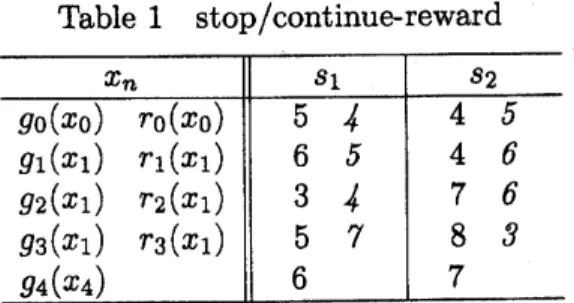
(i) $\tau\in \mathcal{T}_{0}^{4}$ (4)

where the $\mathrm{s}\mathrm{t}\mathrm{o}\mathrm{p}/\mathrm{c}\mathrm{o}\mathrm{n}\mathrm{t}\mathrm{i}\mathrm{n}\mathrm{u}\mathrm{e}$-reward $\{g_{0},g_{1},g_{2}, g_{3}, g_{4};r_{0}, r_{1},r_{2}, r_{3}\}$is given in Table 1, and the

tran-sition matrix is symmetric $(p=q=1/2)$. Let

us

find

an

optimal stopping time by solving

recursive equation.

Table 1 $\mathrm{s}\mathrm{t}\mathrm{o}\mathrm{p}/\mathrm{c}\mathrm{o}\mathrm{n}\mathrm{t}\mathrm{i}\mathrm{n}\mathrm{u}\mathrm{e}$-reward

$x_{n}$ $s_{1}$ $s_{2}$ $x_{n}$ $s_{1}$ $s_{2}$ $g\mathrm{o}(x_{0})$ $r_{0}(x_{0})$ $g_{1}(x_{1})$ $r_{1}(x_{1})$ $g_{2}(x_{1})$ $r_{2}(x_{1})$ $g_{3}(x_{1})$ $r_{3}(x_{1})$ $g_{4}(x_{4})$ 5

₄

6 5 3

₄

5 7 6 4 5 4 6 7 6 8 3 7

It is shown that the total number of stopping times $\{f_{m}(n)\}$ for $m$-state $n$-stage model

satisfies the recursive relation ([6])

$f_{m}(n+1)$ $=$ $1+(f_{m}(n))^{m}$

$f_{2}(m)$ $=$ $1+2^{m}$.

There exist $f_{2}(4)=677$stopping times for twO-state $(m=2)$ fo$\mathrm{u}\mathrm{r}$-stage $(n=4)$ model. Among

them, let

us

find

an

optimal stopping time by solving dynamic programming recursive equation

(3).

First, the forward recursion in Lemma 3.1 generates the following past-value sets :

$\Gamma_{0}=\{(-\infty, \infty)\}$, $\Gamma_{1}=\{(4,4)\}$, $\Gamma_{2}=\{(5,4), (6,4)\}$

$\Gamma_{3}=\{(5,4), (6,4)\}$, $\Gamma_{4}=\{(7,4), (5,3), (6,3)\}$

.

Second, the backward recursion (3) yields an optimal solution in expanded Markov class $\Pi$;

optimal value functions

$v_{0}$, $v_{1}$, $v_{2}$, $v_{3}$, $v_{4}$; $v_{n}=v_{n}(x_{n};\lambda_{n},$$\xi_{n}$

and an optimal policy

$\pi^{*}=\{\pi_{0}^{*}, \pi_{1}^{*}, \pi_{2}^{*}, \pi_{3}^{*}\})$

.

$\pi_{n}^{*}=\pi_{n}^{*}(x_{n};\lambda_{n}, \xi_{n})$.

In fact the optimal solution is calculated

as

follows:

$v_{4}(s_{1}; 7, 4)=7\vee g_{4}(s_{1})-4\Lambda g_{4}(s_{1})=7\vee 6-4\Lambda 6=7-4=3$

$v_{4}(s_{1}; 5, 3)=5\vee g_{4}(s_{1})-3\Lambda g_{4}$(si) $=5\vee 6-3\Lambda 6=6-3=3$

$v_{4}(s_{1}$; 6,3$)$ $=6\vee g_{4}(s_{1})-3\Lambda g_{4}(s_{1})=6\vee 6-3\Lambda 6=6-3=3$ $v_{4}(s_{2}; 7, 4)=7\vee g_{4}(s_{2})-4\Lambda g_{4}(s_{2})=7\vee 7-4\Lambda 7=7-4=3$

$04(\mathrm{s}2)5,3)=5\vee$gA$\{\mathrm{s}2)-$$3\Lambda \mathrm{g}\mathrm{A}\{\mathrm{s}2)=5\vee 7-$$3\Lambda 7=7-$$3$$=4$

$04(\mathrm{s}2)6,3)=6\vee$gA{$\mathrm{s}2)-$ $3$$\Lambda$gA$\{\mathrm{s}2)=6\vee 7-$$3$$\Lambda 7=7-$$3$$=4$

$v_{3}(s_{1}$;5,4$)$ _$=$ ${\rm Max}\{$

$5\vee$$g_{3}(s_{1})-4$$\Lambda g_{3}(s_{1})$

$v_{4}(s_{1}; 5 \vee r_{3}(s_{1}), 4\Lambda r_{3}(s_{1}))\cdot\frac{1}{2}+v_{4}(s_{1} ; 5\vee r_{3}(s_{1}), 4\Lambda r_{3}(s_{1}))\cdot\frac{1}{2}$

$=$ ${\rm Max}\{$

$5\vee g_{3}(s_{1})-4\Lambda g_{3}(s_{1})$

$v_{4}(s_{1}; 5 \vee 7,4\Lambda 7)\cdot\frac{1}{2}+v_{4}(s_{1}; 5\vee 7, 4 \Lambda 7)\cdot\frac{1}{2}$

$=$ ${\rm Max}\{$

$5\vee 5-4\Lambda 5$

$v_{4}(s_{1}$; 7,4$)$$\cdot\frac{1}{2}+v_{4}(s_{1} ; 7, \cdot 4)$

.

$\frac{1}{2}$ $=$ ${\rm Max}\{$

5-4 3$\cdot\frac{1}{2}+3$

.

$\frac{1}{2}$

$=$ ${\rm Max}\{$ 1

$v_{3}(s_{1}$;6, 4$)$ _{$=$ ${\rm Max}\{$}

$v_{4}(s_{1)}.6 \vee r_{3}(s_{1}), 4\Lambda r_{3}(s_{1}))\cdot\frac{1}{2}+v_{4}(s_{1} ; 6\vee r_{3}(s_{1}), 4\Lambda r_{3}(s_{1}))\cdot\frac{1}{2}$

$=$ ${\rm Max}\{$ $6\vee 5-4\Lambda 5$ $v_{4}(s_{1}$;7, 4$)$$\cdot\frac{1}{2}+v_{4}(s_{1}$; 7,4$)$$\cdot\frac{1}{2}$ ${\rm Max}\{$ 6-4 3

.

$\frac{1}{2}+3$

.

$\frac{1}{2}$ $=$ ${\rm Max}\{$ 2 3 $=3$ $\pi_{3}^{*}(s_{1}; 6, 4)=\mathrm{c}o\mathrm{n}\mathrm{t}\mathrm{i}\mathrm{n}\mathrm{u}\mathrm{e}$ $v_{3}(s_{2;}5,4)={\rm Max}\{$ 8-4 3$\cdot\frac{1}{2}+4\cdot\frac{1}{2}$ $=4$ $\pi_{3}^{*}(s_{2};5,4)=\mathrm{s}$ $v_{3}(s_{2}; 6, 4)={\rm Max}\{$ 8-4 3$\cdot\frac{1}{2}+3\cdot\frac{1}{2}$ $=4$ $\pi_{3}^{*}(s_{2}; 6, 4)=\mathrm{s}$ $v_{2}(s_{1} ; 5, 4)={\rm Max}\{$ 5-3 3$\cdot\frac{1}{2}+4$

.

$\frac{1}{2}$ $=3.5$ $\pi_{2}^{*}(s_{1} ; 5, 4)=\mathrm{c}$ $v_{2}(s_{1} ; 6, 4)={\rm Max}\{$ 6-3 3$\cdot\frac{1}{2}+4\cdot\frac{1}{2}$ $=3.5$ $\pi_{2}^{*}(s_{1}; 6, 4)=\mathrm{c}$ $v_{2}(s_{2}; 5, 4)={\rm Max}\{$ 7-4 3$\cdot\frac{1}{2}+4\cdot\frac{1}{2}$ $=3.5$ $\pi_{2}^{*}(s_{2}; 5, 4)=\mathrm{c}$ $v_{2}(s_{2}; 6, 4)={\rm Max}\{$ 7-4 3$\cdot\frac{1}{2}+4$

.

$\frac{1}{2}$ $=3.5$ $\pi_{2}^{*}(s_{2}; 6, 4)=\mathrm{c}$ $v_{1}(s_{1}; 4, 4)={\rm Max}\{$ 6-4 3.5

.

$\frac{1}{2}+3.5$

.

$\frac{1}{2}$ $=3.5$ $\pi_{1}^{*}(s_{1} ; 4, 4)=\mathrm{c}$ $v_{1}(s_{2}; 4, 4)={\rm Max}\{$ 4-4 3.5$\cdot\frac{1}{2}+3.5$

.

$\frac{1}{2}$ $=3.5$ $\pi_{1}^{*}(s_{2}; 4, 4)=\mathrm{c}$ $v_{2}(s_{1} ; 5, 4)={\rm Max}\{$ 5-3 3$\cdot\frac{1}{2}+4\cdot\frac{1}{2}$ $=3.5$ $\pi_{2}^{*}(s_{1}; 5, 4)=\mathrm{c}$ $v_{2}(s_{1} ; 6, 4)={\rm Max}\{$ 6-3 3$\cdot\frac{1}{2}+4\cdot\frac{1}{2}$ $=3.5$ $\pi_{2}^{*}(s_{1}; 6, 4)=\mathrm{c}$ $v_{2}(s_{2}; 5, 4)={\rm Max}\{$ 7-4 3$\cdot\frac{1}{2}+4\cdot\frac{1}{2}$ $=3.5$ $\pi_{2}^{*}(s_{2}; 5, 4)=\mathrm{c}$ $v_{2}(s_{2}; 6, 4)={\rm Max}\{$ 7-4 3$\cdot\frac{1}{2}+4\cdot\frac{1}{2}$ $=3.5$ $\pi_{2}^{*}(s_{2}; 6, 4)=\mathrm{c}$ $v_{1}(s_{1}; 4, 4)={\rm Max}\{$ 6-4 3.5$\cdot\frac{1}{2}+3.5\cdot\frac{1}{2}$ $=3.5$ $\pi_{1}^{*}(s_{1}; 4, 4)=\mathrm{c}$ $v_{1}(s_{2;}4,4)={\rm Max}\{$ 4-4 3.5$\cdot\frac{1}{2}+3.5\cdot\frac{1}{2}$ $=3.5$ $\pi_{1}^{*}(s_{2}; 4, 4)=\mathrm{c}$

$v0(s_{1};-\infty, \infty)={\rm Max}\{$

5-5

3.5

.

$\frac{1}{2}+3.5\cdot\frac{1}{2}$

$=3.5$ $\pi_{0}^{*}(s_{1};-\infty, \infty)=\mathrm{c}$

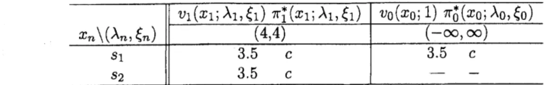
The optimal solution is tabulated in Table 2:

Table 2 optimal solution

$x_{4}\backslash (\lambda_{4}, \xi 4)$

$v_{4}(x_{4;} \lambda 4, \xi 4)$ $(7,4)$ $(5,3)$ $(6,3)$ $s_{1}$ $s_{2}$

3

3 3 3 4 4

$x_{n}\backslash (\lambda_{n}, \xi_{n})$

$v_{1}$$(x_{1} ; \lambda 1, \xi 1)$ $\pi_{1}^{*}(x1; \lambda 1, \xi 1$) $v_{0}(x0; 1)$ $\pi_{0}^{*}(x0; \lambda 0, \xi 0$)

$(4,4)$ $(-\infty, \infty)$ $s_{1}-$ $s_{2}$ $3.\overline{5}\mathrm{c}---$ 3.5 $\underline{c}$ $3.5-$ $-c$

Third,

we see

that an optimal stpping rule $\tau^{*}$ is to stop at state

$s_{2}$

on

stage 3. The rule

implies that

an

optimal decison-maker should continue at any state

on

stages 0, 1, 2 and at

state $s_{1}$ on stage

3

(Figure 1). The maximumexpected value ofrange is $v_{0}(s_{0};-\mathrm{o}\mathrm{o}, \infty)$ $=3.5.$

As is directly verified at thebottom line, the optimal expected value is equal to $E_{s_{1}}[R_{\tau}*]$

.

The

stopping $\mathrm{t}$ime $\tau^{*}$ has

$E_{s_{1}}[R_{\tau}*]=3 \cdot\frac{1}{16}+3\cdot\frac{1}{16}+\cdots+4\cdot\frac{1}{8}=\frac{7}{2}=3.5.$

$\star$ : stop

2

: continue

$\mathrm{o}$ : not reached

67 6 7 6 7 6 7

$R_{n}$ 3 3 4 3 3 4 3 3 4 3 3 4

$\mathrm{p}\mathrm{r}$

.

$\mathit{1}$/16 1/16 1/8 1/16 1/16 1/8 1/16 1/16 1/8 1/16 1/16 1/8

Figure 1 It is optimal to stop at state $s_{2}$

on

stage 3 :

$\tau^{*}$

References

[2] . Bellman and . Denman, Invariant Imbedding, Lect. Notes in Operation Research

and Mathematical Systems, Vol. 52, Springer-Verlag, Berlin, 1971.

[3] $\mathrm{R}.\mathrm{E}$. Bellman and $\mathrm{L}.\mathrm{A}$. Zadeh, Decision-making in a fuzzy environment, Management Sci.

17(1970), B141-B164.

[4] $\mathrm{Y}.\mathrm{S}$

.

Chow, H. Robbins and D. Siegmund, Great Expectations: The Theory

of

Optimal

Stopping, Houghton Mifflin Company, Boston, 1971.

[5] N. Furukawa and S. Iwamoto, Stopped decision processes on complete separable metric

spaces, J. Math. Anal. Appl. 31(1970), 615-658.

[6] H. Hisano, Optimal stopping problemon finiteMarkov chain, Bull. Informatics and

Cyber-netics, 34, No. 2 (2003), 97-104.

[7] S. Iwamoto, Theory

_of

Dynamic Program: Japanese, Kyushu Univ. Press, Fukuoka, 1987.

[8] S. Iwamoto, From dynamic programming to bynamic programming, J. Math. Anal. Appl.

177(1993), 56-74.

[9] S. Iwamoto, On bidecision processes, J. Math. Anal. Appl. 187(1994), 676-699.

[10] S. Iwamoto, Associative dynamic programs, J. Math. Anal. Appl., 201(1996), 195-211.

[11] S.Iwamoto, Maximizing threshold probabilitythroughinvariant imbedding, Ed. $\mathrm{H}.\mathrm{F}$. Wang

and $\mathrm{U}.\mathrm{P}$. Wen, Proceedings of the 8th Bellman Continuum, National Tsing Hua University,

Hsinchu, ROC, Dec, 2000, 17-22.

[12] S. Iwamoto, Fuzzy decision-making through three dynamic programming approaches, $\mathrm{d}$

.

$\mathrm{H}.\mathrm{F}$. Wang and$\mathrm{U}.\mathrm{P}$

.

Wen, Proceedings ofthe 8th Bellman Continuum, National TsingHua

University, Hsinchu, ROC, Dec, 2000, 23-27.

[13] S. Iwamoto, Recursive method in stochastic optimization under compound criteria,

Ad-vances in Mathematical Economics $3(2001)$, 63-82.

[14] S. Iwamoto, K. Tsurusaki and T. Fujita, “On Markov policies for minimax decision

prO-cesses,” J. Math. Anal. Appl., v01.253, nO.1, pp.58-78, 2001.

[15] S. Iwamoto, T. Ueno and T. Fujita, “Controlled Markov chains with utility functions,”

Proc.

_of

Intl Workshop

on

Markov Processes and Controlled Markov Chains, Changsha,

China, August 22-28, 1999, Kuluwer, 2002, pp.135-148. to

appear.

[16] S. Iwamoto and T. Fujita, Stochasticdecision-makingin

a

fuzzyenvironment, J. Operations

${\rm Res}$

.

Soc Japan 38(1995), 467-482.

[17] $\mathrm{E}.\mathrm{S}$. Lee, Quasilinearization an$d$ Invariant Imbedding, Academic Press, New York, 1968.

[18] $\mathrm{A}.\mathrm{N}$

.

Shiryaev, Optimal Stopping Rules, Springer-Verlag, New York, 1978.

[19] M. Sniedovich, Dynamic Programming, MarcelDekker, Inc. NY 1992.

[20] K. Tsurusaki, Extrema-trimmed sum in decision problem, Ed. $\mathrm{H}.\mathrm{F}$

.

Wang and $\mathrm{U}.\mathrm{P}$

.

Wen,

Proceedingsofthe8th Bellman Continuum,National TsingHuaUniversity, Hsinchu,ROC,

Dec, 2000, 2-6.

[7] $\mathrm{S}$

, Iwamoto, Theory

of

Dynamic Program: Japanese, Kyushu Univ. Press, Fukuoka, 1987.

[8] S. Iwamoto, From dynamic programming to bynamic programming, J. Math. Anal. Appl.

177(1993), 56-74.

[9] S. Iwamoto, On bidecision processes, J. Math. Anal. Appl. 187(1994), 676-699.

[10] S. Iwamoto, Associative dynamic programs, J. Math. Anal. Appl., 201(1996), 195-211.

[11] S.Iwamoto, Maximizing threshold probabilitythroughinvariant imbedding, Ed. $\mathrm{H}.\mathrm{F}$. Wang

and $\mathrm{U}.\mathrm{P}$. Wen, Proceedings of the 8th Bellman Continuum, National Tsing Hua University,

Hsinchu, ROC, Dec, 2000, 17-22.

[12] S. Iwamoto, Fuzzy decision-making through three dynamic programming approaches, $\mathrm{d}$

.

$\mathrm{H}.\mathrm{F}$. Wang and$\mathrm{U}.\mathrm{P}$

.

Wen, Proceedings ofthe 8th Bellman Continuum, National TsingHua

University, Hsinchu, ROC, Dec, 2000, 23-27.

[13] S. Iwamoto, Recursive method in stochastic optimization under compound criteria,

Ad-vances in Mathematical Economics $3(2001)$, 63-82.

14] S. Iwamoto, K. Tsurusaki and T. Fhjita, “On Markov policies for minimax decision

prO-cesses,” J. Math. Anal. Appl., v01.253, nO.1, pp.58-78, 2001.

[15] S. Iwamoto, T. Ueno and T. Fujita, “Controlled Markov chains with utility functions,”

Proc.

_of

Intl Workshop

on

Markov Processes and Controlled Markov Chains, Changsha,

China, August 22-28, 1999, Kuluwer, 2002, pp.135-148. to

appear.

[16] S. Iwamoto and T. Fujita, Stochasticdecision-makingin

a

fuzzyenvironment, J. Operations

${\rm Res}$

.

Soc Japan 38(1995), 467-482.

[17] $\mathrm{E}.\mathrm{S}$. Lee, Quasilinearization and Invariant Imbedding, Academic Press, New York, 1968.

[18] $\mathrm{A}.\mathrm{N}$

.

Shiryaev, Optimal Stopping Rules, Springer-Verlag, New York, 1978.

[19] M. Sniedovich, Dynamic Programming, MarcelDekker, Inc. $\mathrm{N}\mathrm{Y}$, 1992.

[20] K. Tsurusaki, Extrema-trimmed sum in decision problem, Ed. $\mathrm{H}.\mathrm{F}$

.

Wang and $\mathrm{U}.\mathrm{P}$

.

Wen,

Proceedingsofthe8th Bellman Continuum,National TsingHuaUniversity, Hsinchu,ROC,