Suzaku
Investigation of Hard X-ray Emission
Associated with the Galactic Center Region
Ken-ichi Tamura
Department of Physics
Graduate School of Science
University of Tokyo
Abstract
In the center region of our Galaxy, the intense diffuse X-ray emission exists. The emission has been observed as X-ray spectra from a hot plasma with a temperature of 108
K, and the mechanism of production has been still a mystery over the past two decade from the discovery. The X-ray observatory, Suzaku, carries the X-ray CCD cameras, XIS, with good energy resolutions and the Hard X-ray Detector, HXD, with high energy band up to several hundreds keV, and therefore, has a large advantage to solve the mystery. Especially, with HXD-PIN which is a component of HXD , we will be able to obtain hard X-ray spectra of the Galactic center diffuse emission if we can estimate the contamination from the hard X-ray sources in the FOV. Hence, we have performed the in-orbit calibrations of the angular response and developed the new method to estimate the contamination.
Contents
1 Introduction 5
2 Review 7
2.1 Overview of the Galactic Center Region . . . 7
2.2 Past X-ray Observations of the Galactic Center Region . . . 9
2.2.1 Ginga results . . . 9
2.2.2 ASCA results . . . 10
2.2.3 Superposition of Dim Point Sources . . . 10
2.3 Non-thermal Hard Tail Associated with the Milky Way . . . 12
2.4 Suzakuresults . . . 13
3 The X-Ray Observatory Suzaku 15 3.1 The Suzaku Spacecraft . . . 15
3.2 X-Ray Telescope (XRT) . . . 17
3.3 X-Ray Imaging Spectrometers (XIS) . . . 22
3.4 Hard X-Ray Detector (HXD) . . . 26
3.4.1 Overview . . . 26
3.4.2 HXD-PIN Detectors . . . 31
3.4.3 In-Orbit Calibration . . . 32
4 Angular Response of HXD-PIN and A New Method for Flux Estima-tion 34 4.1 Angular Response of HXD-PIN . . . 34
4.1.1 Fine-Collimator . . . 34
4.1.2 Angular Response . . . 35
4.2 In-Orbit Calibration of the Angular Response . . . 35
4.2.1 Calibration of Light Axes . . . 35
4.2.2 Fine Tuning of the Angular Response . . . 42
4.3 New Method for Flux Estimation . . . 43
5 Suzaku Observations 50 5.1 Overview . . . 50
5.2.1 Determination of the temperature of the hot plasma . . . 51
5.2.2 Monitoring bright transient hard X-ray sources . . . 51
5.2.3 Observations of molecular clouds . . . 52
5.2.4 Mapping observations . . . 52
5.3 Status of the Observations . . . 52
6 Suzaku Data Analysis and Results 55 6.1 XIS Data Analysis . . . 55
6.1.1 Data Reduction . . . 55
6.1.2 Imaging analysis . . . 55
6.1.3 Analysis of the XIS spectra . . . 59
6.1.4 Surface Brightness Distribution of Soft X-ray . . . 67
6.2 HXD-PIN Data Analysis . . . 70
6.2.1 Data Reduction . . . 70
6.2.2 NXB Modeling . . . 70
6.2.3 Spectral Analysis . . . 71
6.2.4 Spectral Fitting with a Power-law Model . . . 72
6.3 Estimation of Contaminations from Known Hard X-ray Sources . . . 85
6.3.1 Known Hard X-ray Sources in the Galactic Center Region . . . . 85
6.3.2 Flux Estimation of the Hard X-ray Sources with IBIS . . . 86
6.3.3 Spectral Estimation of the Hard X-ray Sources with XIS . . . 95
6.3.4 Flux Estimation of ”1E 1740.7-2942” . . . 96
6.4 Analysis of the Hard X-ray diffuse emission . . . 106
6.4.1 Class A . . . 106
6.4.2 Class B . . . 109
6.4.3 Class C . . . 116
6.4.4 Distribution of Hard X-ray Emission . . . 116
7 Discussion 120 7.1 Brief Summary of the Observational Results . . . 120
7.2 Uncertainties of the Hard X-ray Diffuse Emission . . . 120
7.3 Contributions from the Dim Point Sources . . . 122
7.4 Interpretation of the Hard X-ray Diffuse Emission . . . 123
8 Conclusion 125 A Image of Galactic Center Region with Swift 126 B Individual Observational Data 128 B.1 The XIS spectra and the IBIS fluxes of the bright point sources . . . 128
Chapter 1
Introduction
The intense iron line emission concentrating in the center of our Galaxy has been observed in X-ray band with previous X-ray satellites. This emission often interpreted as diffuse hot plasma with a high temperature of ∼ 6 keV being confined in the galactic center region. Despite of repeated observations and numerous efforts to solve the origin of this diffuse hot plasma, over the past two decades from the discovery of the emission, both ”How the hot plasma has been created?” and ”Why the hot plasma can stay there?” have been mysteries.
In addition, diffuse X-ray emissions from the Galactic plane and bulge have been also observed. From these regions, non-thermal diffuse emissions have also been discovered. However, no conclusions of the emission mechanisms have been obtained. From energetics point of view, the origin of hot plasma confined in the Galactic Center Region is of great importance in modern high energy astronomy. Recently, a symptom of the non-thermal emission has been reporeted from the analysis of the XIS data, (e.g. Koyama et al. 2007), which is the CCD sensor onboard Suzaku.
Suzakuis the fifth Japanese X-ray observatory which has two detector systems. One is XIS, instruments with X-ray CCD cameras, which covers the energy range of 0.2–12 keV. The other detector, HXD, is a collimated detector which features the narrowest field-of-view and the lowest background among recent collimator-type hard X-ray detectors. These features give large advantages to observations for the Galactic center region in which many hard X-ray sources, giant molecular cloud and possible the Galactic center diffuse emission are mixed with each other.
analysis and result of the XIS and HXD data, and the estimation of the contaminations from the hard X-ray sources to the HXD fluxes. In Chapter 7, we discuss the Suzaku
Chapter 2
Review
2.1
Overview of the Galactic Center Region
The Galactic center is the closest galactic nucleus of a spiral galaxy, and hence numer-ous observations have been performed on this region. The central half kiloparsec region around the Galactic Center is an extremely complex region containing a variety of astro-physical activities: cold and warm molecular clouds, star cluster/formation, supernova remnants (SNRs), and HII regions, to name a few. Therefore, this region have been
attracting many researchers in wide-band wavelengths, from radio to very high energy gamma-ray.
Figure 2.1: Velocity integrated (-200 to 200 km s−1) CS J=1-0 emission in
the Galactic center region, obtained with 45 m telescope at Nobeyama Radio Observatory (Tsuboi et al. 1999). The data have been convolved with a 60” Gaussian.
The structures of the molecular clouds, the fountainhead of star formation activities and hot plasmas eventuated, have been mapped with CO and CS lines in the radio wave-length. As shown in figure 2.1, it is clear that they show a strong concentration around the center of Galaxy as a form of giant molecular clouds involved in a continuous ridge extended along the Galactic plane. The compact and luminous nuclear region produces
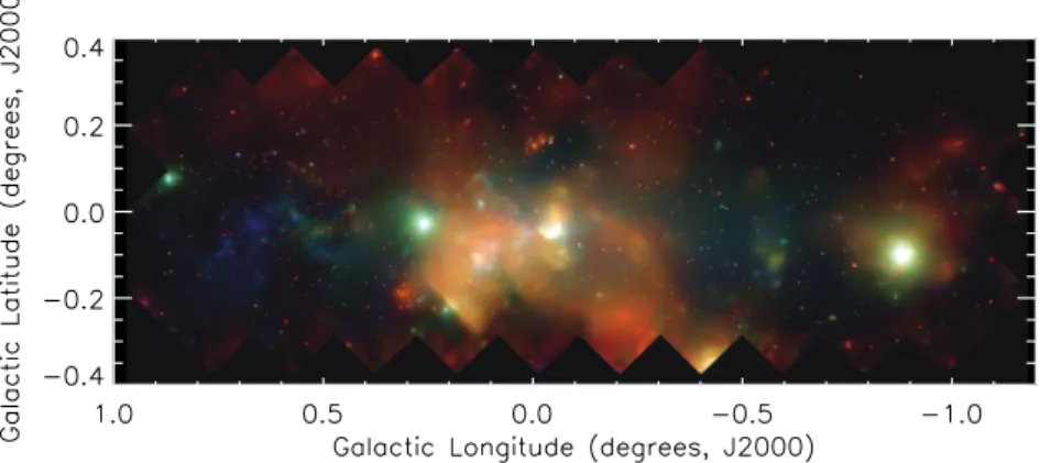
Figure 2.2: A mosaic image obtained with a survey of Spitzer Space Tele-scope/IRAC observations of the central 2×1.5 degrees (265×200 pc) of the Galaxy at 3-8µm.
rougly 10% of the molecular gas content. Overlaid on this global structure, some peculiar structures such as the expanding molecular ring, a center lobe which are often explained as a remnant of huge explosive events, and the radio arc and plumes possibly resulted as a local consolidation of the magnetic field, have been observed (Kaifu et al. 1972, Yusef-Zadeh et al. 1984, Tsuboi et al. 1985).
The highest spatial resolution and sensitivity large-scale map made to date of the Galactic Center at mid-infrared wavelengths has been recently obtained with theSpitzer
2.2
Past X-ray Observations of the Galactic Center
Region
2.2.1
Ginga
results
Based on the discovery of the Fe-K line emission by Tenma (Koyama et al. 1986), an extensive survey of the Fe-K line was performed along the Galactic plane using the Large Area Counter (LAC) aboardGinga, with a filed-of-view of 1◦
.0×2◦
.0 FWHM (Yamauchi et al. 1990). Through the iron line survey observations, Yamauchi et al. discovered a remarkable condensation of the iron line intensity near (≤ 2◦
) the Galactic center, as shown also in figure 2.3. They reported that the shape of this region is an ellipse of 1◦
.8×1◦
.0 tilted by 21◦
with respect to the Galactic plane, and the typical temperature is about 10 keV. The total thermal energy of hot plasma in this region is estimated as (4-8)×1053 ergs, and the total mass of hot gas (1-2)×104M
⊙ . Possible explanations
of this hot gas concentration includes the integrated emission of star forming regions, supernova explosions in the tenuous ambient medium or a single large explosion at the Galactic center. However, definite conclusion is not yet obtained.
2.2.2
ASCA
results
ASCA has been utilized extensively to survey the Galactic center region, and many discrete sources have been resolved from the complex diffuse emission. Figure 2.4 shows the very central region of the Galaxy obtained withASCA (Koyama et al. 1996; Sakano et al. 2000). At the most center, within the 1◦
.8×1◦
.0 ellipse discovered by Ginga ??,
ASCA found a narrower region of 3′ ×2′
centering on Sgr A∗
where the X-ray surface brightness becomes maximum. The energy spectrum of the diffuse emission from the entire ∼1 square degree were characterized by many emission lines from helium-like and hydrogen-like ions of Si, S, Ar, Ca, and Fe, with a continuum described by a thermal bremsstrahlung of ≥ 10 keV (Koyama et al. 1996; Maeda et al. 1998).
Figure 2.4: X-ray image of the Galactic center in 2-10 keV band obtained with theASCA
SIS (Koyama et al. 1996).
Figure 2.5: Hard X-ray (3-10 keV) image of the Galac-tic center region obtained with
ASCA (Sakano 2000).
2.2.3
Superposition of Dim Point Sources
Against the opinion that the diffuse X-ray emissions in the Galactic center region are truly diffuse emissions, another opinion is supported that the diffuse X-ray emissions can be explained by superposition of a lot of dim X-ray point sources. Since 2000, X-ray imagers with good spacial resolutions of 0.5′′
Figure 2.6: X-ray image of the Galactic center region with Chandra.
Figure 2.7: Distribution of X-ray point sources in the Galactic center region detected with Chandra.
number density of the discovered sources (Log-N log-S) even if the detection limit becomes better. While, 90 % of the discovered sources are estimated to be Cataclysmic Variables (CVs). The spectra from the CVs are represented by the thermal bremsstrahlung with a temperature of 10 – 40 keV, and therefore can explain the X-ray spectra obtained with
2.3
Non-thermal Hard Tail Associated with the Milky
Way
Another important scientific prospect obtained withGingais the discovery of thehard-tail
in the GRXE energy spectra as shown in figure 2.8 (Yamasaki et al. 1996a, Yamasaki et al. 1996b, Yamasaki et al. 1997). They discovered that the GRXE spectra obtained with the
Ginga LAC cannot be explained adequately with a single-temperature plasma emission, and obtained the best fit with two emission components, a thin thermal plasma of 3.1±1.4 keV and an additional power-law component of photon index ∼1.6±1.1. Since a single power-law extrapolation of thehard-tail connects smoothly to the diffuse Galactic softγ -ray spectrum (right panel of figure 2.8) which is thought to arise via bremsstrahlung from low-energy cosmic electrons, we presume that some acceleration process is continuously supplying these electrons around the Galactic plane.
Figure 2.9: The soft X-ray spectrum of the Galatic center region with Suzaku.
2.4
Suzaku
results
We review the following two papers before this thesis based on the analysis of theSuzaku
observational data of the Galactic center region. These observations have been performed in the test observational term (within a year from the launch in 2005), and 5 positions of |l|<1.0◦
have been observed.
Koyama et al. (2007c) have performed the precise plasma diagnosis utilizing the ob-servational data (|l| < 0.3◦
,|b| < 0.2◦
) of the X-ray CCD sensors (XIS). They show that the hot plasma is in ionization equilibrium from the energy of the line center and the temperature is 6.5 keV from the line ratio. While, the continuum component of the XIS spectrum is explained by a thermal bremsstrahlung of > 10 keV. Hence, they suggest that there is another component explained by a power-law model, that is the non-thermal emission, from this contradiction (Figure 2.9). However, the spectral shape of the power-law component is not determined at all in only the soft X-ray band.
Koyama et al. (2007c) also show that the Galactic diffuse X-ray emission can not be explained by only the superposition of dim point sources from spatial distributions. Figure 2.10 shows the surface brightness distribution of 6.7 keV line compared with the distribution of integrated point sources fluxes. Since these scale lengths are clearly different with each other, they suggest that the diffuse emission can not be explained by the point sources even if dimmer sources are detected with more sensitive imagers in the future.
Figure 2.10: The 6.7 keV line fluxes distribution obtained bySuzaku(squares). And, the integrated point source fluxes in the 4.7 – 8 keV band are plotted by the crosses.
and HXD and shown that the power-law component which is suggested by Koyama et al. (2007c) extends to 40 keV. However, there are a lot of hard X-ray point sources in the region of |l| < 1.0◦
, and therefore, the systematic errors of the estimations of the contamination from the point sources are large. Hence, the spectral shape of the power-law component can not be determined precisely. Moreover, the hard X-ray surface brightness distribution can not be obtained from only the observational data of|l|<1.0◦
since the Galactic diffuse X-ray emission is considered to extend to |l|= 2◦
from the 6.7 keV line distribution (Maeda 1998).
These results suggest the existence of non-thermal emission in center area of the Galactic center region. The investigation of the hard X-ray emission from the region close to the Galactic center is very important. In this thesis, we extend the analysis of the Suzaku observational data to the position of |l|= 2◦
Chapter 3
The X-Ray Observatory
Suzaku
3.1
The
Suzaku
Spacecraft
The fifth Japanese X-ray astronomy satellite,Suzaku(Mitsuda et al. 2007), was launched on 10 July 2005 with the M-V launch vehicle from Uchinoura Space Center of Japan Aerospace Exploration Agency (JAXA). After the launch,Suzakufirst deployed the solar paddles and the extensible optical bench (EOB), and performed∼10 days of the perigee-up orbit maneuver to get into a near circular orbit of 570 km altitude with an inclination of 31◦
. The orbital period of the satellite is about 96 minutes.
The schematic view and the side view of theSuzakuspacecraft are shown in Figure 3.1 and Figure 3.2, respectively. The five sets of X-ray mirrors are mounted on top of the EOB and five focal plane detectors and a hard X-ray detector are mounted on the base panel of the spacecraft. The spacecraft weight at launch was 1706 kg and its length is 6.5 m along the telescope axis after the deployment of the EOB. The electronics boxes of both the spacecraft bus and the scientific instruments are mounted on the side panels of the spacecraft. The attitude is stabilized by four sets of reaction wheels with one redundancy, while the attitude is measured by three gyroscopes and two star trackers. The spacecraft pointing accuracy is ∼ 0′
.24 with a stability better than 0′
.022 per 4 sec (a half of typical exposure time of CCD cameras). The pointing direction of the X-ray telescope presently has additional uncertainty and temporal variations due to thermal distortion of the spacecraft structure (Serlemitsos et al. 2007). The normal mode of operations will have the spacecraft pointing in a single direction for at least 1/4 day, which corresponds to a good observation time interval of ∼10 ks. With this constraint, most targets will be occulted by the Earth for about one third of each orbit, but some objects near the orbital poles can be observed nearly continuously. Observations are also interrupted by passages of the South Atlantic Anomaly (SAA), in which the particle background drastically increases.
Figure 3.1: A schematic picture of the Suzaku satellite in orbit. (Courtesy of ISAS/JAXA)
(FI; energy range 0.4–12 keV) CCDs and the other is back-illuminated (BI; energy range 0.2–12 keV). Each XIS sensor is located in the foci of a X-ray telescope (XRT; Serlemit-sos et al. 2007) The second instrument is the non-imaging, collimated detector for higher energies, Hard X-ray Detector (HXD; Takahashi et al. 2007). The HXD extends the bandpass of the Suzaku observatory by more than an order of magnitude with its 10– 600 keV bandpass. The last instrument, X-Ray Spectrometer (XRS; Kelley et al. 2007) is the first orbiting X-ray microcalorimeter spectrometer. The early verification phase of the mission demonstrated that the instrument was working properly and that the cryo-gen consumption rate was low enough to ensure a mission lifetime exceeding three years. However, the XRS is no longer operational since the liquid He cryogen was completely vaporized two weeks after opening the dewar guard vacuum vent. The XRS and the XRT dedicated to it will not be discussed further in this thesis.
3.2
X-Ray Telescope (XRT)
TheSuzakuX-Ray Telescopes (XRTs) are thin-foil-nested Wolter-I type telescopes, which are also utilized in ASCA (Tanaka, Inoue, & Holt 1994), XMM-Newton (Jansen et al. 2001),Swift(Gehrels et al. 2004), and some other missions. These are grazing-incidence reflective optics consisting of compactly nested, thin conical elements. The XRT ofSuzaku
is made of very thin (∼178 µm) foils to achieve light weight and high throughput, with moderate imaging capability in the energy range of 0.2–12 keV. Four XRTs onboard
Suzaku (XRT-I0 to XRT-I3) are used for the XIS.
A photograph of an XRT is shown in Figure 3.3. An XRT is a cylindrical structure, having the following layered components:
1. a thermal shield at the entrance aperture to avoid temperature gradient;
2. a pre-collimator mounted on metal rings for stray light elimination;
3. a primary stage for the first X-ray reflection;
4. a secondary stage for the second X-ray reflection;
5. a base ring for structural integrity and interface with the EOB of the spacecraft.
All these components, except the base rings, are constructed in 90◦
segments, called “quadrants”. Four of the quadrants are coupled together by interconnect-couplers and also by the top and base rings. The telescope housings are made of aluminum for an opti-mal strength to mass ratio. Each reflector consists of a substrate also made of aluminum and an epoxy layer that couples the reflecting gold surface to the substrate.
Table 3.1 summarizes the specifications and the characteristics of the XRTs. The angular resolutions of the XRTs are about 2.0′
Figure 3.3: ASuzaku X-ray telescope (XRT).
angular resolution does not significantly depend on the energy of the incident X-ray in the energy range ofSuzaku, 0.2–12 keV. The effective areas are typically 440 cm2 at 1.5 keV
and 250 cm2 at 7 keV per telescope. The focal lengths are 4.75 m. Individual XRT
quadrants have their own focal lengths deviated from the design values by a few cm. The optical axes of the quadrants of each XRT are aligned within 2′
from each other. The field of view for XRTs, defined as the full-width-at-half maximum (FWHM), is about 20′
at 1 keV and 14′
at 7 keV.
The optical axis of each XRT was determined by observing the Crab Nebula at various off-axis angles. Hereafter all the off-axis angles are expressed in the detector coordinate system (Det-X, Det-Y) (Ishisaki et al. 2007). The result of the determination is shown in Figure 3.4. Since the optical axes moderately scatter around the origin, it was adopted as the XIS-nominal position. On the other hand, the optical axis of the HXD-PIN detector deviates by ∼ 5′
in the negative Det-X direction. Because of this effect, the observation efficiency of the HXD-PIN at the XIS-nominal position is reduced to ∼90% of the on-axis value, and another pointing position, HXD-nominal position, is provided for HXD-oriented observations at (Det-X, Det-Y) = (−3′
.5,0′
). At the HXD-nominal position, the effciency of the XIS is ∼88%.
Verification of the imaging capability of the XRTs were made with the observation of a moderately bright point source, SS Cyg. Figure 3.5 shows the image, Point-Spread Function (PSF), and Encircled-energy fraction (EEF) of the XRT modules. The total exposure time used here is 9.1 ks. The obtained HPD is 1′
.8, 2′
.3, 2′
.0, and 2′
.0 for XRT-I0, 1, 2, and 3, respectively.
It is known that ASCA observations were sometimes hampered by X-rays arriving from sources out of the field of view, which we refer to as stray light. This stray light makes observations of crowed regions like the Galactic center difficult. In order to reduce the effect of the stray light, Suzaku XRT has a pre-collimator in front of the XRT.
22–September 16 at off-axis angles of (Det-X, Det-Y) = (±20′
,0′
), (0′
,±20′
), (±50′
,0′
), and (0′
,±50′
). An example stray-light image is shown in the right panel of Figure 3.6. This image was taken with XIS3 in the 2.5-5.5keV band when the Crab Nebula was offset at (Det-X, Det-Y) = (−20′
,0′
). The left and central panels show simulated stray light images without and with the pre-collimator, respectively, of a monochromatic point source of 4.5keV being located at the same off-axis angle. The ghost image seen in the left half of the field of view is due to the stray light. Although the stray light cannot be completely diminished at an off-axis angle of 20′
, the center of the field of view is nearly free from stray light.
Table 3.1: Specifications/Characteristics of the XRTs onboard Suzaku
Focal Lenth 4.75 m Weight/Telescope 19.3 kg Geometrical Area/Telescope 873 cm2
Field of Viewa 17′
at 1.5 keV 13′
at 8 keV
Effective Areab 440 cm2 at 1.5 keV
250 cm2 at 8 keV
Angular Resolutionb 2′
(HPD)
a
Diameter of the area within which the effective area is more than 50% of the on-axis value.
b
Figure 3.4: Locations of the optical axis of each XRT module in the focal plane determined from the observations of the Crab Nebula. The dotted circles are drawn every 30′′
in radius from the XIS-nominal position.
Figure 3.5: Image, Point-Spread Function (PSF), and Encircled-energy frac-tion (EEF) of the XRT modules in the focal plane. The EEF is normalized to unity at the edge of the CCD chip. With this normalization, the HPD of the XRT-I0 thorough I3 is 1′
.8, 2′
.3, 2′
.0, and 2′
Figure 3.6: Focal plane images formed by stray light. The left and middle panels show simulated images of a monochromatic point-like source of 4.51keV locating at (Det-X, Det-Y) = (−20′
,0′
) in the cases of without and with the pre-collimator, respectively. The radial dark lanes are the shades of the alignment bars. The right panel is the in-flight stray image of the Crab Nebula in the 2.5-5.5keV band located at the same off-axis angle. The unit of the color scale of this panel is counts per 16 pixels over the entire exposure time of 8428.8s. The counting rate from the whole image is 0.78± 0.01 counts s−1
including background. Note that the intensity of the Crab Nebula measured with XIS3 at the XIS-nominal position is 458 ± 3 counts s−1 in the same
3.3
X-Ray Imaging Spectrometers (XIS)
The X-ray Imaging Spectrometers (XISs; Figure 3.7), X-ray sensitive silicon charge-coupled devices (CCDs), are operated in a photon-counding mode, similar to those used in the ASCA SIS, Chandra ACIS, and XMM-Newton EPIC. In general, an X-ray CCD converts an incident X-ray photon into a charge cloud, with the magnitude of charge proportional to the energy of the absorbed X-ray. This charge is then shifted out onto the gate of an output transistor via an application of time-varying electrical potential. Thus, a voltage level (pulse height) proportional to the energy of the X-ray photon is read out.
The four Suzaku XISs are designated as XIS0, XIS1, XIS2, and XIS3, located in the focal plane of XRTs; XRT-I0, XRT-I1, XRT-I2, and XRT-I3, respectively. In an XIS camera, there is a single CCD chip with an array of 1024×1024 pixels, and covers an 17′
.8×17′
.8 region on the sky. The pixel size is 24 µm×24 µm, and the the size of the whole chip is 25 mm×25 mm. One of the XISs, XIS1, uses a back-illuminated (BI) CCD, while the other three use front-illuminated (FI) CCDs. Since the BI CCD has no gate structure on its illuminated side, XIS1 more sensitive to soft X-rays than the other XISs (see Figure 3.8). Table 3.2 is the summary of the specifications and characteristics of XIS.
Since the Suzaku launch on 2005 July 10, the XIS has been working properly, and, the on-board performance and the strong points of the XISs have been demonstrated. The features of Suzaku XISs are its low non-X-ray background (NXB) and good energy resolution over a wide spectral band. These features play important roles in observations of diffuse and low surface brightness sources like our Galactic center region.
Figure 3.9 shows the NXB spectra of FI and BI sensors when the XIS observes the dark (night) Earth. The data obtained during the passage thorough the SAA and events in the calibration source area (the 2 corners) have been excluded. The lines at 5.9 keV and 6.5 keV are due to scattered X-rays from the calibration sources. Other than these, many lines, Kα of Al, Si, Ni, Kβ of Ni, and Lα, Lβ, and Mα lines of Au are detected. Thanks to the low-Earth orbit of Suzaku, the NXB is fairly low, especially for the FI CCDs.
The flux of NXB depends on the cut-off rigidity (COR): the FI fluxes in the 0.4–12 keV band are about 0.2 counts s−1 and 0.1 counts s−1 for the COR of 4–6 GV and 12–14 GV,
respectively, while the BI fluxes in the same COR bands are about 0.6 counts s−1 and
0.3 counts s−1, respectively. Thus for the most accurate NXB subtraction, the data
should be selected so that the COR distribution of the NXB observation is the same as that in the source observation.
Figure 3.7: A Suzaku XIS sensor.
and Ni XXVII, Kβ lines of Fe I, Fe XXV, and Fe XXVI, and even Kγ lines of Fe XXV and Fe XXVI are found above ∼ 7 keV. This demonstrates reliable NXB subtraction and superior energy resolution. These capabilities of the XIS enable us to perform line-resolved imaging studies even of low surface brightness sources.
In general, the energy resolution of X-ray CCDs in orbit have got worse due to the radiation damage. In order to recover the degradation of the energy resolution, Suzaku
XIS has a capability of a spaced-row charge injection (SCI), and the SCI technique has been applied since 2006 December. The radiation damage makes “traps” in X-ray CCD pixels. These traps obstruct the event transfer, which causes the degradation. If charges are put in front of X-ray events, these charges works as “sacrificial” events. Therefore, they fill the traps and the X-ray events are transferred smoothly, and the energy resolution can be restored. This is the principle of the SCI.
Figure 3.8: Effective area of one XRT + XIS system, for both FI (XIS0, 2, 3) and BI (XIS1) CCDs.
Figure 3.9: The night Earth spectra with the BI and FI CCDs.
Figure 3.11: Comparison of the He-like Fe Kα line spectrum between with the SCI and without the SCI.
Table 3.2: Specifications/Characteristics of XIS
Field of View 17′
.8×17′
.8
Energy Range 0.2–12 keV
Format 1024×1024 pixels Pixel Size 24 µm×24µm
Energy Resolution ∼ 130 eV (FWHM) at 5.9 keV
Effective Areaa 330 cm2 (FI), 370 cm2 (BI) at 1.5 keV
160 cm2 (FI), 110 cm2 (BI) at 8 keV
Readout Noise ∼ 2.5 electrons (RMS) Time Resolution 8 s (with Normal Mode)
a
3.4
Hard X-Ray Detector (HXD)
3.4.1
Overview
The Hard ray Detector (HXD; see Figure 3.12) is a non-imaging, collimated hard X-ray instrument sensitive in the ∼10 keV to ∼600 keV band. The characteristics of the HXD is summarized in Table 3.3. Since the background level sets the sensitivity limit in the hard X-ray band, the HXD is designed to minimize the background by its improved phoswich (acronym for PHOSphor sandWICH) configuration for the energy region above 40 keV and the adoption of newly-developed thick silicon PIN diodes for the energies below 70 keV.
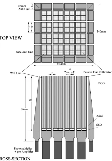
Figure 3.13 is the schematic drawing of HXD sensor. Two key techniques are used here: well-type active shield and compound eye configuration.
• Well-type active shield
In phoswich counters, two crystals with different decay times are used for the de-tection part (faster decay time) and the shielding part (slower decay time), and both signals are extracted by a single photomultiplier. The improvement is that the shield is shaped as well, so that it also acts as an active collimator (well-type active shield). This narrows the field of view of the phoswich counter without ad-ditional passive material, and results in the main detection part having an active shield of almost 4π of its surrounding (well-type phoswich counter). In the HXD, well-type shield provides very efficient shielding for the the PIN diodes, which are also located at the bottom of the well and are read out independently.
• Compound eye configuration
HXD is modular designed, consisting of a number of units. Each well-type phoswich counter unit has a simple shape and operates at a modest count rate by itself. In the HXD, we increase the photon collecting area by placing individual units in a matrix. In this configuration, each unit also becomes an active shield for adjacent units (Compound eye configuration). It is also useful to reduce the possible dead time if parallel processing of each unit could be implemented. For additional shielding for the outer most units, thick anti-coincidence counters are placed surrounding the well units.
The HXD sensor consists of 16 phoswich counters each with 4 silicon PIN diodes, and 20 surrounding anti-coincidence shield counters. The main detection part of phoswich counters is a Gadolinium silicate crystal (GSO; Gd2SiO5(Ce)) buried deep in the bottom
of the Well-shape Bismuth germanate crystal (BGO; Bi4Ge3O12) (hereafter we refer it
Figure 3.12: Hard X-ray Detector (HXD) onboard Suzaku
shield counters (Anti-counter units) are also made of BGO. All the 16 Well-counter units and 20 Anti-counter units work independently. Numbering of the Well-counters and Anti-counters, which is frequently referred to in this thesis is shown in Figure 3.14. The Anti-counters also work as an excellent gamma-ray burst monitor with its large effective area for sub-MeV to MeV gamma-rays. The gamma-ray burst location determination is about 5◦
.
✂✁☎✄✝✆✞✆
✟✡✠☞☛
✌✎✍✏✒✑✒✓
✠☞✔✕☛
✖✕✗✒✏✙✘✏ ✆✛✚☎✜
✘✍✢
✜
✍✓✤✣
✥
✢✒✣✓✧✦★ ✆ ✢✜✍✩✍✓✣ ✪✬✫✮✭✰✯✰✱✕✲✬✳
✴✶✵✸✷✺✹✻✹✽✼☎✹✛✾✶✴❀✿❂❁✒✷✬❃ ❄❅ ❆❇
❈❂✓✜✜✒❉✡❊✍✘ ❋☎●❍✒■❑❏✡▲✒▼●✒◆☞▲✒●▼
★ ❊✘✍❉☞❊✍✘
✖◗P✧❘❘✍❙✕✓❯❚❱✍❊✓ ❖ ✏✜✜✍✆ P✘✏✂✣ ❄❅
❲❆❳❆ ❲❆❳❆
❨
❩❅
❬❭❪
✝✁☎✄✂✆✞✆
❬❫❪❴❵❴
T00 T01 T02 T03 T04 T10 T20 T21 T22 T23 T24 T30 T11 T34 W00 W01 W10 W11
T12 T33 W03 W02 W13 W12
T13 T32 W30 W31 W20 W21
T14
T31 W33 W32 W23 W22 P0 P1
P2 P3
PIN in Well 1 unit Configuration of Sensor Units (Top View)
Y
X
Figure 3.14: Numbering of the Well and Anti counter units when HXD Sensor is viewed from the top. There are 16 Well-counter units from W00 to W33 and 20 Anti-counter units from T00 to T34. The Y-direction corresponds to the direction toward Sun when the HXD is mounted to the spacecraft.
GSO PIN diode assembly BGO BGO ✁ ✁ ✁ ✂✄✂ ✂✄✂ ✂✄✂ ☎✄☎ ☎✄☎ ☎✄☎ PMT Plastic
Rubber Plastic and Rubber
Carbon fiber reinforced plastic (CFRP)
Fine collimator
Figure 3.16: Total effective area of the HXD detectors, PIN and GSO, as a function of energy. Photon absorption by materials in front of the device is taken into account.
Table 3.3: Specifications/Characteristics of HXD
Field of View 34′ ×34′
(. 100 keV) 4◦
.5×4◦
.5 (&100 keV) Energy Range 10–600 keV
– PIN 10–70 keV – GSO 40–600 keV Energy Resolution
– PIN ∼ 4.0 keV (FWHM) – GSO 7.0/√EMeV % (FWHM)
Effective Area ∼160 cm2 at 20 keV ∼260 cm2 at 100 keV
7750 p+ n+ Al SiO2 p+ p+ Guard Ring Al n+ 2490 2000 Polyimide 10750 bonding wire
Silicone rubbre
Ceramics case
Silicone rubbre
Figure 3.17: A photograph (left) and a schematic picture (right) of a HXD-PIN diode
3.4.2
HXD-PIN Detectors
The silicon PIN diodes cover the lower energy region of the HXD bandpass, from 10 keV to 70 keV. For the HXD data, only the data from PIN detectors are used in this thesis. Figure 3.17 shows the photograph and the schematic picture of the PIN diode. The geo-metrical area of the PIN diode, including the guard ring structures, is 21.5 mm×21.5 mm with a thickness of 2 mm. The leakage current is less than 2.2 nA at the operation condi-tions (500 V and −20 ◦
C). In order to minimize the background gamma-ray contamina-tion for the PIN, we have selected low-background material for cables and package. The adoption of ceramic with a purity higher than 96% for the PIN package was required to avoid continuum gamma-ray background due toβ-decay electrons from potassium in the material.
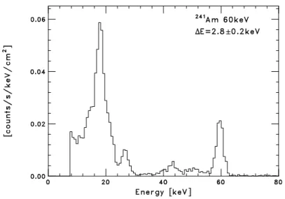
Figure 3.18 demonstrates the superior performance of the PIN diode. This is a spec-trum of X-rays/gamma-rays from 241Am obtained with a PIN diode on the ground. As
shown in this figure, an energy resolution of 2.8 keV was achieved and the energy thresh-old was ∼10 keV. The energy resolution of the PIN preamplifier is 1.0 keV in a load-free condition; this degrades to 1.6 keV by the capacitive noise, and another 1.0 keV is due to the leakage current noise. The remaining ∼ 2.1 keV is possibly caused by electronic noise.
Field of view (FOV) of the HXD-PIN is collimated with fine collimators in order to reduce contamination of Cosmic X-ray Background (CXB) and point sources which are not targets. Having a narrow field of view is the most effective method to reduce the background contamination. For this purpose, passive shields called ”fine collimators” are inserted to the BGO well-type collimator above the PIN diodes. The fine collimator is made of 50 µm thick phosphor bronze sheets arranged to form a square array of 8 × 8 channels each of 3 mm width and 300 mm length. The fine collimators confine the FOV of PIN diodes even narrower than that restricted by the active shield of BGO. The FOV defined by the fine collimators is 34.2′
×34.2′
Figure 3.18: A PIN spectrum of241Am obtained on the ground. The
temper-ature is−20◦
C
triangle with FWHM of 34.2′
. Calibrations of the angular response is described precisely in the next chapter.
3.4.3
In-Orbit Calibration
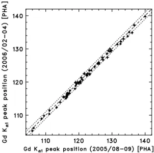
Calibrations of gains and energy scale and measurements of energy resolution are essential in constructing the instrumental response function, which in turn is needed to reconstruct incident spectra from the observed pulse-height distributions. Before the launch, the energy scales of the 64 PINs were precisely measured using the standard gamma-ray sources, within ∼1% accuracy (Takahashi et al. 2007). These energy scales are not expected to change significantly after the launch, because neither the charge collection efficiency of the PIN diodes nor the capacitance of the charge sensitive amplifiers is sensitive to the environmental changes. Nevertheless, the energy scale is so important that it should be accurately reconfirmed using the actual data.
In order to determine the energy scale, line features in the spectrum are useful. Since the line emissions can be rarely observed from celestial objects in the bandpass of HXD-PIN, X-ray line emissions generated within the detector are utilized. Figure 3.19 illus-trates the events used for the calibration. When an X-ray photon is absorbed in GSO, a fluorescent X-ray photon from gadlinium (Gd-Kα: 42.7 keV) sometimes escape from the
BGO Well
GSO PIN
X-rays
Gd-K
Absorption
BGO Well
GSO PIN
X-rays
Bi-K Absorption
Figure 3.19: Illustration of an event in which Gd-K X-ray is detected with a PIN diode (left) and in which Bi-K is detected.
Chapter 4
Angular Response of HXD-PIN and
A New Method for Flux Estimation
Calibrations of the angular response is essential in estimating fluxes of point sources in the FOV of HXD-PIN, especially in care of crowded region like the Galactic center. In this chapter, first, we describe in-orbit calibrations of the angular response. Then, we introduce a method to estimate the flux of point sources in the FOV by use of differences of individual optical axes of 64 fine-collimetors of the PIN detector.
4.1
Angular Response of HXD-PIN
4.1.1
Fine-Collimator
In the energy range of the PIN diode, the dominant background component is the cosmic X-ray background. Therefore, having a narrow FOV is the most effective method to reduce the background contamination. For this purpose, passive shields called “fine collimators” are inserted in the BGO well-type collimator above the PIN diodes. The fine collimator is made of 50µm thick phosphor bronze sheets arranged to form a square array of 8× 8 square channels each of 3 mm width and 300 mm length.
Both the BGO collimator and the fine collimator define the FOV of the Well-counter unit. Because of the finite thickness, the FOV changes with the photon energy. Below
∼ 100 keV, the fine collimators confine the FOV of PIN diodes much narrower than the BGO collimator and define a 34′
×34′
Full-Width Half-Maximum (FWHM) square FOV. Above ∼ 100 keV, the fine collimators become transparent and the BGO active collimator defines a 4.5o
× 4.5 o FWHM square opening.
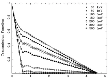
The angular response of HXD-PIN is determined by the fine-collimator . Functional form the angular transmission of the fine collimator is plotted in Figure 4.1 with respect to the incident angle of X-rays, and we call this as an angular response of HXD-PIN. The function is determined to be almost a triangle shape with a width of 34.2′
of 300 mm of the opening part of the fine collimator. Hereafter, we define a direction at which the transmission becomes maximum as the ”light axis” of the fine-collimator.
4.1.2
Angular Response
Angular response, the transmission efficiency of the collimator, is one of most important issues of calibration. Without accurate number, we would not be able to derive the flux from sources.
The angular response of the fine collimator depends on the direction of its light axis with respect to the pointing direction of the satellite. If the alignment of the collimator is different with each other, we have to take these differences into account when we calculate the angular response of the PIN detector. Meanwhile, the angular response dose not depend on the energy range of HXD-PIN (below 80 keV) (Figure 4.1), therefore we do not have to include the energy dependency in this thesis. In the actual observational data, the angular response is characterized by the equation;
R[i] = F[i]
f , (4.1)
whereRis the angular response for each fine collimator,iis ID of the PIN corresponding to the collimator, F is the flux arrived at the surface of the PIN detector and f is the expected flux when we locate the target in the direction of light axis.
The functional form of the angular response with respect to the pointing direction of the satellite is defined by the shape of the fine collimator as schematically shown in Figure4.2. In the figure, an effective area is indicated as ”not-shadowed” region, and therefore the ratio of observed flux and the real flux corresponds to the ratio of the area of ”not-shadowed” region divided by the total effective area of the PIN detector.
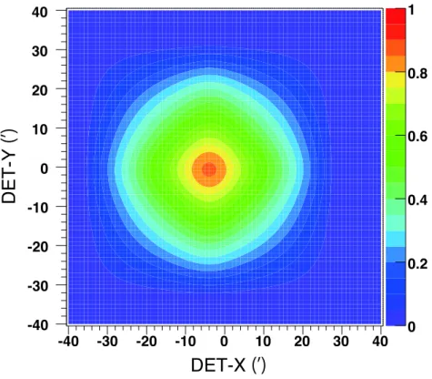
Once we obtain an offset of the light axes of the fine-collimators from the pointing direction of the satellite, we are able to calculate the angular response for a source from any directions in the FOV by using a triangle-shaped function defined by the mechanical structure and its thickness. Figure 4.3 shows the 1-D profile of the angular response for the position of the point source in the FOV. And, Figure 4.4 shows the 2-D one.
4.2
In-Orbit Calibration of the Angular Response
4.2.1
Calibration of Light Axes
Although the directions of 64 fine collimators have been finely adjusted before launch, there still remain slight (∼ 1′
Figure 4.1: Angular transmission function of the fine collimator calculated at azimuth angle of 0◦
. The 0◦
Side view
Bottom view
(X-axis)
1 pixel / 8 x 8 pixels
of
fine collimator
Shadow
Target
Light axis
Shadow of X-axis (Bx)
Shadow of Y-axis (By)
A
A
ARF
1.0
Light axis of the PIN
Nominal position of the satellinte
34.2
ARF[
i
]
Target
Figure 4.3: Schematic perspective of determination of the ratio.
-40 -30 -20 -10 0 10 20 30 40
-40 -30 -20 -10 0 10 20 30 40
0 0.2 0.4 0.6 0.8 1
D
ET
-Y
()
DET-X ( )
Figure 4.5: Distribution of light axes of the individual fine-collimators mea-sured in the ground test.
Before the launch, the light axes of the 64 fine collimators have been measured by means of optical laser light and radio-isotope sources. Figure 4.5 shows their angular offsets measured by scanning 31 keV gamma-ray line from 133Ba. We define the origin
(δx = 0, δy = 0) at the mean of the offsets of each light axes of 64 fine-collimators. According to the ground calibration, the collimators are aligned up with an accuracy of 3.5′
(FWHM). This ensures an effective transparency of 90%, when a target is placed at the mean direction of optical axes of the 64 fine-collimators.
Distribution of the light axes, shown in Figure 4.5, leads to deviation of effective area for each PIN detector with a range of ∼ 20 % . When we sum up the flux measured by each PIN detector, we have to apply these factors to the flux obtained from individual detectors. In the ground tests, it was difficult to prepare a bright and parallel hard X-ray beam which is necessary to calibrate the light axes precisely. In addition, the light axes may have changed by the vibrations of the launch and thermal stress. Therefore, we have to perform in-orbit calibration of the light axes.
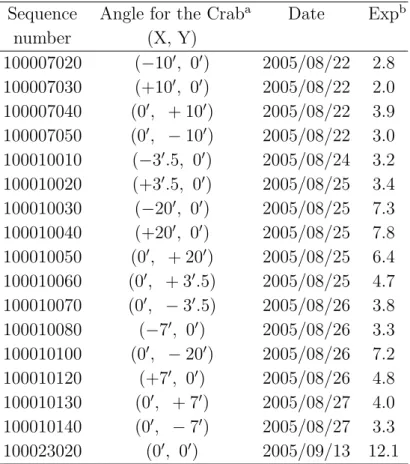
We used Crab Nebula as a calibration target, since the source is bright in the hard X-ray band from 10 keV up to 50 keV and fluxes of the source are known to be stable in time. To obtain the actual shape of the transmission function used to reconstruct the angular response for each collimator, we have performed multiple observations of the Crab with several offset angles separated with ∼10′
.
Table 4.1 shows the observation log of the Crab-scan observations. In order to deter-mine the light axes of the individual fine-collimetors, we have to know the peak positions of the triangle along both the X-axis and the Y-axis. Therefore, we performed the scan-ning observation along both axes with offset angles of 0′
,±3.5′
,±7.0′
,±10.0′
and±20.0′
We determined these pitches such that we could obtain the peak position with a sufficient accuracy compared to the size of the triangle of 34.2′
(FWHM).
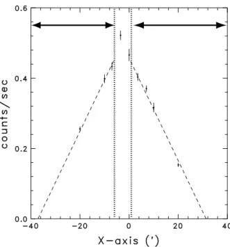
Counting-rate distribution is shown in Figure 4.6. with an energy range of 15–40 keV. This energy rage is chosen to reduce systematic uncertainties to the angular response, due to possible contamination of thermal noise around 10 keV. We apply the standard screening criteria (ver. 2.0) which is described in chapter 6.
Table 4.1: Summary of the Crab observations of various angles.
Sequence Angle for the Craba Date Expb
number (X, Y) 100007020 (−10′
, 0′
) 2005/08/22 2.8 100007030 (+10′
, 0′
) 2005/08/22 2.0 100007040 (0′
, + 10′
) 2005/08/22 3.9 100007050 (0′
, −10′
) 2005/08/22 3.0 100010010 (−3′
.5, 0′
) 2005/08/24 3.2 100010020 (+3′
.5, 0′
) 2005/08/25 3.4 100010030 (−20′
, 0′
) 2005/08/25 7.3 100010040 (+20′
, 0′
) 2005/08/25 7.8 100010050 (0′
, + 20′
) 2005/08/25 6.4 100010060 (0′
, + 3′
.5) 2005/08/25 4.7 100010070 (0′
, −3′
.5) 2005/08/26 3.8 100010080 (−7′
, 0′
) 2005/08/26 3.3 100010100 (0′
, −20′
) 2005/08/26 7.2 100010120 (+7′
, 0′
) 2005/08/26 4.8 100010130 (0′
, + 7′
) 2005/08/27 4.0 100010140 (0′
, −7′
) 2005/08/27 3.3 100023020 (0′
, 0′
) 2005/09/13 12.1
a
The offset angles for the Crab in the satellite nominal coordinate.
b
Effective exposure of HXD-PIN data.
We determine individual peak positions by fitting the distribution of the counting rate along X-axis and Y-axis with the triangle of a width of 34.2′
(FWHM). Since the actual shape of the angular response can not be modeled by a triangle function around the top, we perform fitting with the data excluding points within 3.5′
Figure 4.6: An example of the count rates distribution extracted from the scanning observations of the Crab. The PIN ID is W00P3.
The “light axis of HXD-PIN”, namely, the average direction of 64 light axes, at which the total transparency of fine-collimetors become maximum, is determined as (X, Y) = (−4.03′
,−0.62′
) and root mean squares of the distribution are 1.58′
for the X-axis and 1.70′
for the Y-axis. The difference of light axes between HXD-PIN and XIS exists, since detected photons with HXD-PIN decreases by 13% in the case that the nominal axis of the satellite is directed at the target source. Therefore Suzaku team prepared the second nominal position of the satellite ”HXD-nominal” with the position of (X, Y) = (−3.5′
,−0.0′
) in addition to the first that of ”XIS-nominal” with (0.0′
,0.0′
).
4.2.2
Fine Tuning of the Angular Response
Utilizing the measured directions of the light axes for all fine-collimetors, we reconstruct an actual shape of the angular response as shown in Figure 4.8. The figure is created by plotting 64 points from each the Crab scanning observation. The energy range is 16–40 keV. The sky coordinate positions of the individual data points correspond to directions of the light axes of the individual fine-collimators in the actual observations. The upper panel of the figure is the plot drown along RA-axis of sky coordinate and the lower panel DEC-axis. The plots of the RA and DEC-axis are created with the observational data of the Crab scanning observations along Y and X-axis respectively. The vertical axis is detected counting rates during the observation the individual PINs. We note that the correspondence of X-axis and Y-axis with axes of RA and DEC is inverted since the roll angles of these observation are ∼ 90◦
. The center of the triangle certainly agree with the position of the Crab.
In Figure 4.8, the counting rates are corrected with difference of relative effective areas in the energy range of 16−40 keV. The effective area of each PIN diode is calculated from a thickness of a depletion layer of the detector. The PIN diodes of HXD-PIN are as thick as ∼ 2.0 mm and a bias voltage around 700 V is required to obtain full depletion of Si (Ota et al. 1999). At the nominal operation voltage of∼ 500 V, the actual thickness of the depletion layer could vary among the 64 PINs. The thicknesses of the individual PIN diodes were tuned using an observational data of the Crab (Tanaka 2007). And then, the difference of the thicknesses should be taken into account when the energy response of the individual PINs. Using the individual energy responses (ver. 2007-09-14), we extracted the relative effective areas as shown Figure 4.9. The relative effective areas were normalized to 1.0 when the average of 64 PINs was set to 1.0. The counting rates of Figure 4.8 were calculated with dividing the raw counting rates by the relative affective areas.
each fine collimator. The round shape near the top of the triangle could be explained by small differences of directions, ∼1′
, among 8×8 pixels in ”one” fine-collimator. The narrower width could be explained by surface roughness and distortion (∼ 50 µm) of the phosphor bronze used in the fine-collimator. We use the function extracted from the actual data as the angular response for point sources in this thesis, as shown in Figure 4.10. The map of the corrected angular response summed with 64 PINs is also shown in Figure 4.11.
4.3
New Method for Flux Estimation
Distribution of corrected flux at different offset angles, shown in Figure 4.8 , suggests that the accurate estimation of a flux of a point source in the FOV is possible by using the distribution of the count rate from individual PIN detectors, if the position of the sources is given. The flux, the height of the triangle, can be calculated by solving a simple linear equation which consists of position of the peak and leaning of the data points. The calculation is afford to say as a simple imaging with a large PSF of 33′
and small FOV of several squares of minutes. We have developed a method to estimate the flux of the source even if the FOV is filled with another uniform emission such as the diffuse emission of the Galactic center region. As a summary, the flux estimation method introduced here is to solve the linear equations explained above for the individual PINs. When the FOV is filled with an uniform emission, an equation is provided as follows;
F[i] =R[i]f+B, (4.2)
where F is a flux arrived at the surface of the PIN detector, R is angular response, i is PIN’s ID, f is expected flux in the case that the target exists in the direction of light axis and B is an uniform background emission. In this equation, known parameters are
F[i] and R[i], while unknown parameters f and B. Since the number of the unknown parameters is two, we are able to obtain values of the variables as long as two individual equations of equation 4.2 from the observational results of two PINs’ are given.
Since statistics of the two PIN’s fluxes are usually not enough to calculate f of the target, we utilized equations obtained from summed data of 64 PINs. In order to obtain the most effective statics, we define an equation
near
∑
i
F[i]−
far
∑
i
F[i] =
near
∑
i
R[i]f−
far
∑
i
R[i]f, (4.3)
where ”near” and ”far” are groups of PINs whose light axes are nearer and farer from a direction of the target. The flux of the target is given as below equation,
f = (
near
∑
i
F[i]−
far
∑
i
F[i]) /(
near
∑
i
R[i]−
far
∑
i
It is assumed that the uniform background emission is constant for the individual PINs. An example of a correlation between R and counting rates of the individual PINs are shown in Figure 4.12. The figure was created by using the actual data of one of the Crab scanning observations. The sequence number of the observation is ”10007020” whose position to the Crab is (X,Y) = (+3.5’, 0′
). The position is counter side of the light axis of HXD-PIN for the Crab. It is expected that we are able to clearly confirm the correlation between the ratio of the angular response and the actual counting rates using the data of the position, in which the lean of the function is constant and the statics of the counting rates is good. In the figure, the horizontal axis means the ratio of the angular response of the individual PINs to the targets in the FOV. Meanwhile, the vertical axis means the counting rates of the individual PINs corrected with the relative effective areas. An energy range of the counting rates is 16−40 keV. We confirmed that there are clear correlations between the ratio and the counting rates.
In order to confirm if the method can be utilized realistically, we calculated estimation limits of this method. An uncertainty of the calculated flux is determined by statistics of the NXB and fluxes from the source. And then, the detection limits are defined by the significance for the statics of the NXB.
At the observation of ”10007020”, an expected counting rate of the NXB is 0.26 counts/sec in an energy range of 16–40 keV, for example. From the rate, counting rate of each PIN is calculated to 4 ×10⁻³ counts/sec/PIN roughly. We assumed this rate as
the typical counting rates and calculated the limits of the flux estimation method. When an exposure of an observation is EXP sec, an integration of count of the NXB is equal to 4 ×10⁻³×EXP counts/PIN. At the equation 4.4, the flux of the source is calculated
by the counting rate F from the target and the ratio of the angular response R. In the actual analysis, F is calculated by subtracting counting rate of the NXB from the detected counting rate. Therefore, statics ofF are determined by the statics of the NXB and counting rate form the target. And then, the statical uncertainty of the component in the equation, ∑
iF[i], is calculated by
√
32×(4×10−3 ×EXP) = √0.13×EXP since
the number of the PIN is 32 for each group. And then, changed to a unit of counts/sec,
√
0.13/EXP. Finally, the uncertainty of the estimated flux, ∆f, is calculated as follows,
∆f =√2×0.13/EXP / (
near
∑
i
R[i]−
far
∑
i
R[i]). (4.5)
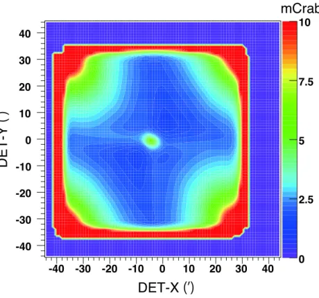
The ratioR is calculated for each position, and a map of ∆f calculated for each meshed position is shown in Figure 4.13. We created the figure assuming that the exposure is 40 ksec. The units of the map is ”mCrab” which is corresponds to 4.6×10⁻⁴counts/secin
the energy range of 16–40 keV. In an observation of exposure of 40 ksec, the uncertainty at the most sensitive position is ∼ 1 mCrab at 1 σ significance. In this figure, the sensitivity in the center of FOV is worse since the difference of counting rates between two groups,(∑near
i F[i]−
∑f ar
Figure 4.8: Reconstructed shape of the angular response with the Crab scan-ning observations.
response While, the sensitivity around the end is worse since the transmittance is small and then the static of the detected counting rate is not good.
Utilizing this method, we estimated the flux of the Crab using the results of the scanning observations listed in Table 4.1. Figure 4.14 shows the estimated fluxes of the Crab compared among the scanning observations for X and Y-axis. We confirmed that the fluxes are estimated adequately within statistical uncertainty. Since the direction of light axis of HXD-PIN is (X,Y) = (−4.03′
,−0.06′
) and the rounding top of the angular response is positioned at the direction, the uncertainty of the observation in (X,Y) = (−3.5′
,0′
) is worse.
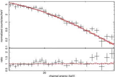
Performing the flux estimation method every energy bin, we are able to obtain spec-trum of the target source. Figure 4.15 shows spectra of the Crab extracted with the estimation method and regular means from the observational data of ”100023020” whose nominal position of the satellite is XIS-nominal of (X, Y) = (0′
,0′
Figure 4.9: Distribution of the relative effective area among PINs’.
-40 -30 -20 -10 0 10 20 30 40 -40
-30 -20 -10 0 10 20 30 40
0 0.2 0.4 0.6 0.8 1
DET-X
( )
D
ET
-Y
()
Figure 4.11: Actual angular response of the HXD-PIN which is summed up responses of 64 PINs’.
Near
Far
-40 -30 -20 -10 0 10 20 30 40 -40
-30 -20 -10 0 10 20 30 40
0 2.5 5 7.5 10
DET-X
( )
D
E
T
-Y
()
mCrab
Figure 4.13: Detection limit of the simple imaging method with an exposure of 40 ksec.
0
.1
1
0
.2
0
.5
2
5
n
o
rma
liz
e
d
co
u
n
ts/
se
c/
ke
V
20
0
.5
1
1
.5
2
ra
ti
o
channel energy (keV)
Chapter 5
Suzaku
Observations
5.1
Overview
Since the launch of Suzaku in 2005, we have performed thirty five observations the Galac-tic Center region (|l| < 2◦
.0,|b| < 0.5◦
). Most of the observations were performed in 4 terms; from 2005-09-23 to 2005-10-12, from 2006-02-20 to 2006-03-01, from 2006-09-09 to 2006-10-12 and from 2007-03-03 to 2007-03-18. The first two terms were done in SWG (Science Working Group) phase and the last two were done in AO-1 (1st Announcement of Oppotunity) phase. Total net exposure is amount be ∼1 Msec . The details of the observations, exposures, dates and positions of the observations, is listed in table 5.1. The position of each pointing is show in figure 5.1 as an exposure map of the XIS.
5.2
Strategy of the observations
first time.
The observation of the Glactic Center Region was originally proposed as a big project for the entire Suzaku team, and there are several objectives in its 1 Ms observation. Here we summarize four strategies related to the investigation of the non-thermal component in the wide band specra.
5.2.1
Determination of the temperature of the hot plasma
In order to study an excess of the non-thermal emission, we need to constrain the shape of spectra of the thermal emission. The first step is to determine the temperature of the plasma and its distribution. The temperature is given by an intensity ratio between 6.7 keV and 6.9 keV lines, which corresponds to K-α lines from He-like and H-like Fe ion in optically thin hot plasma. Based on the previous observations of the Galactic Center Region withGinga,ASCA,Chandra andN ewton, we define the region of interest to be
|l|<2◦
.0,|b|<0.5◦
. By taking the size of the FOV of the XIS into account, we divide the region into two. Also, in order to increase the robustness of the temperature determined from the two Fe line emissions, we observed the same position twice for some cases. There are four observations in September 2005. One of the two positions was observed again as a calibration of the XIS in March 2006. In total, we have five observations, in which data is mostly used to determine the properties of thermal spectrum which characterize the Galactic Center Region. Exposures of the individual observations were decided to be large enough to resolve the two Fe line emissions clearly and obtain a detailed temperature of the hot plasma. Roll angles during each observation were optimized to the requirement came from by the sun angle.
5.2.2
Monitoring bright transient hard X-ray sources
In the Galactic Center region, there are many transient X-ray and hard X-ray sources. Although the collimated instrument, like HXD, has high sensitivity especially for the diffuse emission, it would be difficult to extract fluxes from point sources in the FOV. The smallest FOV of HXD-PIN allows us to reliably estimate the contamination of hard X-ray point sources, since expected number of sources in the FOV is small for most of cases and we have simultaneous data from XIS. The XIS data can be used to constrain the source acticity. Most of known sources in the Galactic Center Region has changes the flux with time scale of a week, therefore, the aim is satisfied with these sources if we could monitor the source activity with XIS during this time scale. The second strategy is, therefore, to monitor especially bright hard x-ray sources with the XIS.
spectra and flux.
5.2.3
Observations of molecular clouds
In the Galactic Center region, there are several giant molecular clouds which are known to be a strong emitter of neutral Fe line of 6.4 keV. X-ray emission from the clouds itself is an important topic to study the activities of the Galactic Center, but these are out of scope of this thesis. In the Galactic Center Region observation, significant amount of exposure time was given in the observations of the cloud, ”Sgr B2”, ”Sgr C” and ”Sgr D”. For the HXD, bright hard x-ray sources are relatively small in these regions, we use the data set from the observations of molecular clouds to study the distribution of hard X-ray emission in both positive and negative side of galactic latidude.
5.2.4
Mapping observations
In order to study the origin of hot plasma and also to investigate the hard X-ray emission associated with the Galactic Center Region, it is important to cover the entire region continuously.
According to the spacial distribution of 6.7 keV line emissions which indicate an existance of the hot plasma, a scale height of the Galactic diffuse emission is predicted to be∼0◦
.5 from a We, therefore, adopted∼0◦
.2 for a pitch of positions of observations which is smaller than the scale height if we take the FOV of the XIS into account. We gave a priority to cover to move the FOV along the Galactic longitude since the 6.7 keV line emissions are distributed wider along the Galactic plane than that along the Galactic bulge. These mapping observations were defined to the 4th starategy.
There are some other observations in the Galactic Center region, which were proposed under different motivation, but we included those data in this thesis if the data can be accessed.
5.3
Status of the Observations
Table 5.1. Observations of the Galactic Center region.
Step Sequence Positiona Start Expb SCIc 400V-HVd
number l b (UTC) (ks) on/off unit
1 100027010 0.057 -0.074 2005-09-23 07:07:00 34.9 off – 100027020 -0.247 -0.046 2005-09-24 14:16:00 33.4 off – 100037010 -0.247 -0.046 2005-09-29 04:25:00 36.7 off – 100037040 0.057 -0.074 2005-09-30 07:41:00 33.0 off – 501046010 -0.167 0.333 2007-03-10 14:43:00 22.9 on W0,W1 2 100027030 -0.441 -0.389 2005-09-24 11:05:00 1.7 off –
100027040 -0.446 -0.067 2005-09-24 12:40:00 1.6 off – 100027050 0.328 0.010 2005-09-25 17:27:00 1.7 off – 100037020 -0.441 -0.389 2005-09-30 04:29:00 2.1 off – 100037030 -0.446 -0.067 2005-09-30 06:05:00 2.5 off – 100037050 0.328 0.010 2005-10-01 06:21:00 2.0 off – 3 100037060 0.637 -0.095 2005-10-10 12:07:00 65.9 off – 100037070 1.000 -0.100 2005-10-12 07:05:00 8.6 off – 500018010 -0.569 -0.093 2006-02-20 12:30:00 43.8 off – 500019010 -1.091 -0.041 2006-02-23 10:50:00 11.0 off – 501039010 0.780 -0.160 2007-03-03 12:05:00 84.6 on W0,W1 501040010 0.607 0.072 2006-09-21 17:21:00 49.8 on W0 501058010 1.300 0.200 2007-03-14 05:00:00 46.8 on W0,W1 501059010 1.167 0.000 2007-03-15 18:55:00 49.6 on W0,W1 501060010 1.500 0.000 2007-03-17 05:06:00 50.2 on W0,W1 4 500005010 0.428 -0.117 2006-03-27 22:40:00 60.4 off –
Table 5.1—Continued
Step Sequence Positiona Start Expb SCIc 400V-HVd
number l b (UTC) (ks) on/off unit
4 501054010 -0.167 -0.333 2007-03-12 08:09:00 21.5 on W0,W1 501055010 -0.5 -0.333 2007-03-12 23:58:00 19.9 on W0,W1 501056010 -0.833 -0.333 2007-03-13 15:40:00 23.1 on W0,W1
aFOV (XIS-nominal) center position.
bEffective exposure of the HXD-PIN data.
cXIS’s SCI mode.
dHXD-PIN’s units whose bias voltage was 400 V.
0 500 1000 1500 2000 2500
0.000 0.500
1.000 1.500
2.000 359.500 359.000 358.500 358.000
-1 .0 00 -0. 8 0 0 -0 .6 0 0 -0.4 0 0 -0 .2 0 0 0 .2 0 0 0 .4 0 0 0 .6 0 0 0 .8 0 0 1 .0 0 0 100027010 100027030 100027040 100027020 100027050 100037010 100037020 100037030 100037050 100037060
100037070 500018010
500019010 500005010 100048010 501040010 501008010 501009010 501049010
501050010 501051010 501052010 501053010
501057010 501039010
501046010 501047010 501048010
501054010 501055010 501056010 501058010
501059010 501060010
100037040
Chapter 6
Suzaku
Data Analysis and Results
In this chapter, we describe data reduction procedures and results on the analysis. Firstly, we analyze the data obtained with XIS and HXD-PIN independently. Secondly, the contaminations from the hard X-ray sources are subtracted from the HXD-PIN spectra. Thirdly, we perform the joint analysis of the XIS and HXD-PIN spectra to investigate the non-thermal emission from the Galactic center region.
6.1
XIS Data Analysis
6.1.1
Data Reduction
We have used Suzakudata sets processed by theSuzaku data processing pipeline version 2.0. together with the calibration data set of version 2007-08-04. We have screened the data set with the standard event selections as follow. We have filtered out data obtained during passages through the South Atlantic Anomaly (SAA) since Non X-ray Background (NXB) of the XIS was large enough to saturate the sensor. And the data has been filtered with elevation angle to the Earth’s limb below 5◦
, or with elevation angle to the bright Earth’s limb below 20◦
, in order to avoid the possible contamination of emission of the scattered solar X-rays from the earth. We have filtered out a part of imaging area of the CCD chips where calibration isotopes irradiate. These area corresponds to two corners of each chip. Hot pixels of the chips are also removed by following the standard procedure. These criteria are summarized in Table 6.1. We have not filtered out the data with the Cut Off Regirity (COR).