Bartlett correction to the likelihood ratio test for MCAR with two-step monotone sample
Nobumichi Shutoh
Graduate School of Maritime Sciences, Kobe University email address: [email protected]
Takahiro Nishiyama
Department of Business Administration, Senshu University
Masashi Hyodo
Department of Mathematical Sciences, Graduate School of Engineering, Osaka Prefecture University
Assuming that two-step monotone missing data are drawn from a multi- variate normal population, this paper derives the Bartlett-type correction to the likelihood ratio test for Missing Completely At Random (MCAR) which plays an important role in the statistical analysis of incomplete datasets. The advantages of our approach are confirmed in Monte Carlo simulations. Our correction drastically improved the accuracy of the type I error in Little’s (1988) test for MCAR, and performed well even on moderate sample sizes.
Keywords and Phrases Asymptotic expansion; Bartlett correction;
Missing completely at random; Monotone missing data.
Mathematics Subject Classification 62H15; 62E20.
1 Introduction
When statistically analyzing missing data, the missing mechanism is important be- cause it justifies or invalidates the application of the statistical method. Although specifying the missing mechanism in a likelihood function is a natural approach, misspecifying the missing mechanism leads to severe bias in the result. Even when the missing mechanism can be specified exactly, its parameters must be estimated along with the population parameters. These missing mechanism parameters are nuisance parameters.
To conduct a missing data analysis without specifying the missing mechanism, we must determine the ignorability of the missing mechanism. The ignorabolity con- dition holds if the Missing At Random (MAR) and parameter distinctness are both satisfied (for details, see Little and Rubin, 2002). Under ignorability, we can apply methods based on direct maximum likelihood. Typically, the estimators returned by direct maximum likelihood have no closed forms, implying that their exact ditribu- tion cannot be theoretically obtained (see e.g., Srivastava and Carter, 1986). Kanda and Fujikoshi (1998) obtained closed forms and the exact distribution of the direct maximum likelihood estimators in monotone missing data, a special case that often manifests as dropout of the samples. However, the obtained estimators take more complicated forms than those of complete data. In the last two decades, researchers have developed direct likelihood methods for statistically analyzing monotone miss- ing data with ignorability. As discussed in Hao and Krishnamoorthy (2001), Batsidis et al. (2006), and Tsukada (2014), most of these methods were developed for two- step monotone missing data under the following settings; for j = 1, . . . , N, observe i.i.d. copies of X ∼ Np(µ,Σ) denoted by x′j = (x′1j, x′2j). For j = N1+ 1, . . . , N, x2j are missing from N2 ≡ N −N1 samples, where x2j is a (p−d)-dimensional partitioned sample vector with p > d >0.
More simply, for small sample sizes with missing data, we can apply statistical methods to complete datasets after listwise deletion, or simpler estimators based
on pairwise deletion. However, in applying these methods to missing data, we must restrict the conditions of the missing mechanism, i.e., Missing Completely At Random (MCAR). To this end, we focus on testing the statistical inference for the satisfaction of MCAR. The classical MCAR test was pioneered by Little (1988). He developed a likelihood ratio test that asymptotically follows the chi- squared distribution under MCAR, which were implemented in statistical software.
An alternative test, based on the generalized least squares criterion, was proposed by Kim and Bentler (2002). Recently, Li and Yu (2015) proposed an approximate test for MCAR under the nonnormal model. However, approximate tests for MCAR tend to fail at small sample sizes. For instance, the false rejection of the MCAR hypothesis in Little’s test (i.e., type I error) is likely to increase on small datasets.
This paper considers a Bartlett-type correction of the likelihood ratio test pr- posed by Little (1988), which dramatically reduces the occurence of type I error without a complicated critical value. The correction is applied to two-step monotone missing data, for which various statistical methods have been developed. Because the test statistic depends not only on the ratio of determinants of Wishart matrices but also on the quadratic form of the difference of the sample mean vectors, we alternatively derive them by Nagao’s (1973) perturbation method.
The remainder of this paper is organized as follows. Section 2 simplifies the test statistic derived by Little (1988) to a form useful for our purpose. Section 3 lists the auxiliary results and derives the main result of this paper. Section 4 demonstrates the advantages of our correction test in Monte Carlo simulations of small sample sizes. Conclusions are presented in Section 5, and the proofs are detailed in Appendix A.
2 Likelihood ratio test statistic for MCAR
This section derives the likelihood ratio test for MCAR. As shown in Li and Yu (2015) of Proposition 1, the MCAR test in this case reduces to the testing of
H : xj i.i.d.
∼ Np(µ,Σ) (j = 1, . . . , N1) and x1j i.i.d.
∼ Nd(µ1,Σ11) (j =N1+ 1, . . . , N)
versus
A: xj i.i.d.∼ Np(µ,Σ) (j = 1, . . . , N1) and x1j i.i.d.∼ Nd(ν1,Γ11) (j =N1+ 1, . . . , N).
At least one of the two equations µ1 =ν1 and Σ11 = Γ11 is violated, where µ and Σ are decomposed as
µ= ( µ1
µ2 )
, Σ =
( Σ11 Σ12
Σ21 Σ22 )
.
Here, µ1 is a d(< p)-dimensional subvector ofµ and Σ11 is a d×d submatrix of Σ.
Little (1988) proposed the likelihood ratio test statistic −2 ln Λ, where Λ = LH(µ,e Σ,e µe1,Σe11)
LA(µ,b Σ,b νb1,bΓ11).
Let LH(µ,e Σ,e µe1,Σe11) and LA(µ,b Σ,b bν1,Γb11) be the likelihoods with maximum like- lihood estimators (MLEs) under H and A, respectively. The MLEs of µ,Σ,µ1,Σ11 under H, denoted by tildes placed over the parameters, were derived by Anderson and Olkin (1985). The MLEs of µ,Σ,ν1,Γ11 under A are distinguished by hat symbols over the parameters.
In the assumed special case of the two-step monotone sample, we have
−2 ln Λ = q+N1[tr(SFΣe−1)−p−ln|SF−1|+ ln|Σe−1|] (2.1) +N2[tr(SL,11Σe−111)−d−ln|SL,11−1 |+ ln|Σe−111|],
where
q = N1(xF −µ)e ′Σe−1(xF −µ) +e N2(x1L−µe1)′Σe−111(x1L−µe1), xF =
( x1F x2F
)
, xℓF = 1 N1
N1
∑
j=1
xℓj, x1L = 1 N2
∑N j=N1+1
x1j,
SF =
( SF,11 SF,12 SF,12′ SF,22
)
, SF,ℓm = 1
N1WF,ℓm, SL,11 = 1
N2WL,11, WF,ℓm =
N1
∑
j=1
(xℓj −xℓF)(xmj −xmF)′, WL,11 =
∑N j=N1+1
(x1j −x1L)(x1j−x1L)′, e
µ =
( µe1 e µ2
)
, µe1 = N1
N x1F +N2
N x1L, µe2 = x2F −Σe′12Σe−111(x1F −µe1), Σ =e
( Σe11 Σe12 Σe′12 Σe22
)
, Σe11 = N1
N SF,11+ N2
N SL,11, Σe12 = Σe11SF,11−1 SF,12, Σe22 = SF,22+SF,12′ SF,11−1 (Σe11−SF,11)SF,11−1 SF,12
for ℓ, m= 1,2.
In a complete dataset, the distribution of the likelihood ratio test statistic is usually invariant under an affine transformationCX, whereC is ap×pnonsingular matrix. Unfortunately, such transformation invariance does not generally hold for two-step monotone sample. However, by restricting C, we can recover a similar property.
Lemma 2.1. Suppose that C is a p×p nonsingular matrix with the block decompo- sition:
C =
( C11 O12 C21 C22
) ,
where C11, C21, and C22 are a d×d constant matrix, a (p−d)×d constant matrix, and a (p−d)×(p−d)constant matrix, respectively. O12 denotes a d×(p−d)matrix filled with zeros. Then, the distribution of the test statistic−2 ln Λis invariant under the transformation X 7→CX.
To simplify the form of the test statistic presented in (2.1), we state an auxiliary lemma. Furthermore, by matrix manipulations such as inverting the matrix via block decomposition (see e.g., Lemma 7 of Shutoh (2012)), we can simplify the form of the likelihood ratio test statistic presented in (2.1).
Theorem 2.2. Suppose that we observe a two-step monotone sample from a mul- tivariate normal distribution; that is, we draw xj (j = 1, . . . , N1) samples from a p-dimensional normal distribution and observe x1j (j =N1+ 1, . . . , N) on the first d characteristics of the same distribution. The likelihood ratio test statistic for H is then obtained as
−2 ln Λ = z′ (1
N(WF,11+WL,11+zz′) )−1
z+N {
ln 1
N(WF,11+WL,11+zz′) + tr[(WF,11+WL,11)(WF,11+WL,11+zz′)−1]−d
}
−N1ln 1
N1WF,11
−N2ln 1
N2WL,11
(2.2)
where
z=
√N1N2
N (x1F −x1L).
Remark 2.3. The test statistic for H obtained by Theorem 2.2 is independent of x2j (j = 1, . . . , N1).
3 Distribution of the test statistic and its Bartlett’s type correction
This section derives the main result of this article, i.e., the Bartlett correction to the MCAR testing based on two-step monotone sample assumed in Section 1. The proof of this result relies heavily on the properties of the likelihood ratio test statistic described in Section 2. In particular, by Lemma 2.1, we can assume that Σ = Ip holds without loss of generality.
For simplicity, we consider the distribution of T obtained by replacing N1, N2 and N with n1 =N1 −1, n2 =N2−1 and n =n1 +n2 in the coefficients of (2.2), respectively:
T = z′ (1
n(WF,11+WL,11+zz′) )−1
z+n {
ln 1
n(WF,11+WL,11+zz′) + tr[(WF,11+WL,11)(WF,11+WL,11+zz′)−1]−d
}
−n1ln 1
n1
WF,11
−n2ln 1
n2
WL,11 .
Note thatWF,11 ∼Wd(n1, Id), WL,11 ∼Wd(n2, Id),z ∼Nd(0, Id), which are mutually independently distributed.
To obtain the asymptotic null distribution of T in a large-sample asymptotic framework for two-step monotone sample:
n1, n2 → ∞, γg = ng
n →cg ∈(0,1) (g = 1,2), (3.1) we rewrite the Wishart matrices with
Y1 = (yij(1)) =
√n1 2 ln
( 1 n1WF,11
)
, Y2 = (yij(2)) =
√n2 2 ln
( 1 n2WL,11
) . The natural logarithm of matrices is defined in Nagao (1973). Furthermore, the symmetry of Y1 and Y2 holds by Lemma 2.1 of Nagao (1973). After some algebra, we obtain
T = T0+ 1
√nT1+ 1
nT2+ 1 n√
nT3+Op(n−2), where t0 =z′z+ trY2−trY21,
T1 = −√
2z′Y1z+
√2
3 trY3−√
2trY1Y2 +2√ 2 3 trY31, T2 = −z′Y2z− 1
2(z′z)2+ 2z′Y21z+1
6trY4− 1
2trY22− 2
3trY1Y3+ 2trY21Y2−trY41, T3 is a homogeneous polynomial of degree 5 in terms of (z, Y1, Y2), and Yi =
∑
gγ1−
i
g 2Ygi for g = 1,2 and i = 1,2,3,4, The subscript g denotes the group of missing patterns in ∑
runs 1–2. As z and Yi’s are independently distributed, the characteristic function of T is given by
φ(t)≡E[exp(itT)] = E(Y1,Y2)[Ez[exp(itT)]].
The expectation with respect to z is described by the following formula:
Ez[exp(itT)] = (1−2it)−d2
∫
Rd
exp(it{trY2−trY21}) [
1 + (it)
√nT1 +1
n {
(it)T2+(it)2 2 T12
}
+ 1
n√ n
{
(it)T3 + (it)2T1T2 +(it)3
6 T13 }
+Op(n−2) ]
ϕ(z;0,(t)1Id)dz,
whereϕ(u;η,Ξ) denotes the probability density function ofu, which follows a mul- tivariate normal distribution and takes parameters (η,Ξ), and (t)i = (1−2it)−i.
Furthermore, using the results of Lemma 2 derived by Hyodo et al. (2015) and the technique stated in Section 7 of Nagao (1973), and extending the results in Section 2 of Nagao (1973), the asymptotic probability density function of Yg (g = 1,2) is obtained as
c∗·etr [1
2(ng−d+ 1)
√ 2
ngYg− ng 2 e
√ 2 ngYg
]
(3.2)
× [
1 + d−1 2
√ 2
ngtrYg+ 1
12ng{(3d2−6d+ 2)(trYg)2+dtrYg2}+Op(n−2) ]
wherec∗is defined in formula (2.5) of Nagao (1973). The probability density function of (Y1, Y2) is expressed as
E(Y1,Y2)[Ez[exp(itT)]] = (1−2it)−f2
∫
Rd(d+1)
[ 1 + 1
√nA1+ 1 nA2
+ 1
n√
nA3+Op(n−2) ]
ϕ(y;0,Ψ)dy where f =d(d+ 3)/2, y′ = (y′1,y′2), y′g = (y11(g), . . . , ypp(g), y12(g), . . . , y(g)p−1,p),
Ψ = Cov(y(a)ij , ykℓ(b)) = 1
2(δikδjℓ+δiℓδjk){(t)1(δab−√
γaγb) +√ γaγb}, A1 = (it)Ez[T1]−
√2 6
∑
g
trYg3
√γg,
A2 = −γ˜
24d(2d2+ 3d−1) + p1 12
∑
g
trYg2 γg − 1
12
∑
g
trYg4 γg − 1
12
∑
g
(trYg)2 γg
+ 1 36
{∑
g
(trYg3)2
γg + 2(trY13)(trY23)
√γ1γ2 }
+(it)Ez[T2] + (it)Ez[T1] (
−
√2 6
∑
g
trYg3
√γg )
+ (it)2
2 Ez[T12],
A3 is the sum of the homogeneous polynomials of degrees 1, 3, 5, 7, and 9 in the elements of (Y1, Y2), δij denotes the Kronecker delta, and ˜γ =∑
gγg−1.
The expectations ofA1 and A3 can now be calculated using the following auxil- iary lemma:
Lemma 3.1. Suppose that z1, . . . , zs are i.i.d. copies of a random variableZ follow- ing a distribution that satisfies E[zjr] = 0 ifr is an odd number and E[zjr]̸= 0 other- wise, for j = 1, . . . , s and r∈N. Furthermore, for k ∈N and ij ∈N (j = 1, . . . , s), we define the set of integer partitions of k:
Pk = {
(i1, . . . , is) ∑s
j=1
ij =k }
and another set
Ek = {
(i1, . . . , is) E
[∏s j=1
zjij ]
= 0,
∑s j=1
ij =k }
.
Then, if k is odd, there exists Pk =Ek.
Proof: If all of the ij’s (j = 1, . . . , s) are even numbers, then k is clearly even also.
Note that E[∏s
j=1zjij] = 0 holds if and only if ij is odd for at least onej. By Lemma 3.1, we have
∫
Rd(d+1)A1·ϕ(y;0,Ψ)dy =
∫
Rd(d+1)A3·ϕ(y;0,Ψ)dy= 0.
Finally, after applying the moments of the multivariate normal random variables to all terms inA2, we obtain the characteristic functionφ(t) and the Bartlett correction to T.
Theorem 3.2. Under the large-sample asymptotic framework stated in (3.1), the characteristic function φ(t) is expanded as
φ(t) = (1−2it)−f2 [
1− d
24nc(˜γ){1−(1−2it)−1} ]
+O(n−2), where c(˜γ) = (2d2 + 3d−1)(˜γ−1) + 6d.
Corollary 3.3. Under the large-sample asymptotic framework stated in (3.1), the distribution function of
TB = (
1− c(˜γ) 6n(d+ 3)
) T
is expanded as Pr[TB ≤x] = Pf(x) +O(n−2), where Pf(x) denotes the distribution function of the chi-squared distribution with f degrees of freedom.
Theorem 3.2 and Corollary 3.3 are completed in the Appendix. Finally, we propose a test based on the Bartlett correction: reject H if TB > χ2f(α), where α is the significance level, and χ2f(α) is the upper 100α% point of the chi-squared distribution with f degrees of freedom. In the next section, we demonstrate that TB better-controls the type I error than −2 ln Λ in a simulation study.
4 Simulation study
In this section, the superiority of our test statistic TB over T is demonstrated in Monte Carlo simulations of type I error correction for selected parameter values.
For this purpose, we simulated the upper 100α% points of the test statistics T and TB, denoted by T(α) and TB(α) respectively, under H. Here, T(α) and TB(α) denote the ⌊r·α⌋-th largest value of T’s and TB’s, respectively, in r replications.
The attained significant levels (ASLs) of the test statisticsT andTBare respectively defined by
ASLT(α) = ♯[T > χ2f(α)]
r , ASLB(α) = ♯[TB > χ2f(α)]
r .
For each case in all simulations, we set r= 1,000,000 and varied α as 0.1,0.05 and 0.01 (corresponding to⌊r·α⌋=r·α= 100,000,50,000 and 10,000).
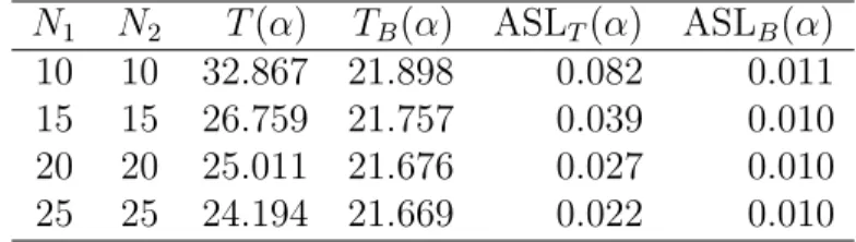
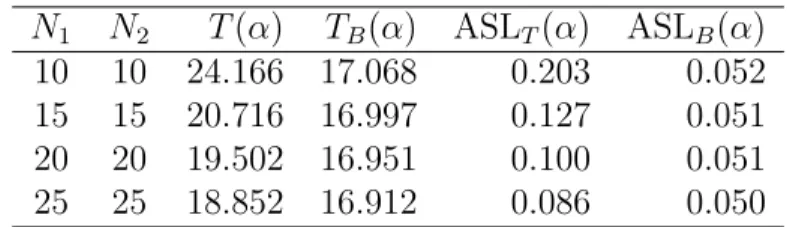
In our first simulation study, we set (p, d) = (4,1),(4,2),(4,3), and assumed equal sample sizes N1 =N2 = 10,15,20,25. We evaluated the ASLB(α) and TB(α) and compared them with ASLT(α) and T(α), respectively. The results are listed in Tables 1–9. In all cases, our test statistic TB outperformed T. Furthermore, the ASL of TB closely approximated α when the sample size is small. In particular, at smaller dimensionalities d, our proposed test clearly performed better than the T statistic.
In our next simulation study, we set (p, d) = (4,2) and N = 50 and 100, with N1/N2 = 1 and 1/4. The ASLB(α) and TB(α) were calculated similarly to the first cases, and the results are listed in Tables 10–12. Again, our test statistic TB consistently outperformed the T statistic. However, when the sample sizes were
unbalanced, the performances of both test statistics were degraded relative to their performances on equal sample sizes.
5 Conclusion
In this paper, we discussed the testing the statistical inference for the satisfaction of Missing Completely At Random (MCAR). If the missing mechanism is MCAR, we can apply statistical methods on the complete dataset after listwise deletion;
otherwise, we can apply simpler estimators based on pairwise deletion. Therefore, MCAR plays a very important role in missing-data handling.
The classical MCAR test was derived by Little (1988), who considered a likeli- hood ratio test statistic that asymptotically distributed as chi-squared distribution under MCAR. However, approximate tests for MCAR perform poorly on small sam- ple sizes. To resolve this problem, we proposed a Bartlett-type correction of the likelihood ratio test proposed by Little (1988), and applied it to two-step monotone missing data. Our proposed test drastically reduced the type I error without com- puting a complicated critical value. Furthermore, in Monte Carlo simulations, the size of the proposed test approximated the nominal significance level even for small sample sizes.
In conclusion, we recommend our proposed test for two-step monotone missing data. A test procedure based on the Bartlett-type correction will be developed for general-monotone missing data in future study.
Acknowledgments
The authors would like to thank Dr. Tamae Kawasaki, Tokyo University of Science, for her help in numerical simulations. The research of the first two authors was supported in part by a Grant-in-Aid for Young Scientists (B) (16K17642, 26730020) from the Japan Society for the Promotion of Science. The third author was funded by Seed Grant Program for Junior Researchers of Osaka Prefecture University.
A Proofs
A.1 Proof of Theorem 2.2
Applying the following formula:
Σ =e
( Id O12 Σe′12Σe−111 Ip−d
)( eΣ11 O12 O21 Σe22·1
)( Id Σe−111Σe12 O21 Ip−d
)
, (A.1)
where Σe22·1 =Σe22−Σe′12Σe−111Σe12, and applying the formula stated in (A.1) toSF, we have
−ln|SF|+ ln|Σe| = −ln 1
N1WF,11 + ln
1
N(WF,11+WL,11+zz′)
. (A.2)
Performing matrix inversion and Σ decomposition, we also obtaine tr(SFΣe−1) = N
N1tr[WF,11(WF,11+WL,11+zz′)−1] + (p−d), (A.3) and
q = z′ ( 1
N(WF,11+WL,11+zz′) )−1
z. (A.4)
Equations (A.2)–(A.4) complete the proof of Theorem 2.2.
A.2 Proofs of Theorem 3.2 and Corollary 3.3
To prove the theorem, we first define J(Y1,Y2)[g(y)] =
∫
Rd(d+1)
g(y)·ϕ(y;0,Ψ)dy, and
Jz[h(y,z)] =
∫
Rd
h(y,z)·ϕ(z;0,(t)1Id)dz,
whereg(y) is a function of the elements ofyandh(y,z) is a function of the elements of Y1, Y2 and z.
Using the result for multivariate normal random vectors, we obtain J(Y1,Y2)[∑
g
trYg2 γg
]
= d
2(d+ 1){(˜γ−2)(t)1+ 2}, J(Y1,Y2)[∑
g
trYg4 γg
]
= d
4(2d2+ 5d+ 5){(˜γ−3)(t)2+ 2(t)1+ 1}, J(Y1,Y2)[∑
g
(trYg)2 γg
]
= d{(˜γ−2)(t)1+ 2}, J(Y1,Y2)[∑
g
(trYg3)2
γg +2(trY13)(trY23)
√γ1γ2 ]
= 3
4d(4d2+ 9d+ 7)[(˜γ−4)(t)3+ 3(t)2+ 1]
+9
2d(d+ 1)2{−(t)2+ (t)1}. Therefore, we have
J(Y1,Y2) [ d
12
∑
g
trYg2 γg − 1
12
∑
g
trYg4 γg − 1
12
∑
g
(trYg)2 γg + 1
36 {∑
g
(trYg3)2
γg +2(trY13)(trY23)
√γ1γ2
}]
= d
48(4d2+ 9d+ 7)(˜γ−4)(t)3− d
48(2d2+ 5d+ 5)(˜γ −6)(t)2 + d
24(d−1)(d+ 2)(˜γ−1)(t)1+ d
24(3d2+ 4d−3). (A.5) By Lemma 2 of Hyodo et al. (2015), we also have
Jz[T2] = −(t)1tr(∑
g
Yg2 )
− 1
2p1(p1+ 2)(t)2 + 2(t)1tr[(∑
g
√γgYg )2]
+1
6tr(∑
g
1 γgYg4
)
− 1
2tr[(∑
g
Yg2 )2]
−2
3tr[(∑
g
√γgYg
)(∑
g
√1γgYg3 )]
+2tr[(∑
g
√γgYg
)2(∑
g
Yg2 )]
−tr[(∑
g
√γgYg )4]
.
As the folowing relationships hold J(Y1,Y2)
[ tr[∑
g
Yg2 ]]
= d
2(d+ 1){(t)1+ 1}, J(Y1,Y2)
[
tr[(∑
g
√γgYg )2]]
= d
2(d+ 1), (A.6)
J(Y1,Y2) [
tr[∑
g
1 γgYg4
]]
= d
4(2d2+ 5d+ 5){(˜γ−3)(t)2+ 2(t)1+ 1}, J(Y1,Y2)
[
tr[(∑
g
Yg2 )2]]
= d
4(2d2+ 5d+ 5){(t)2+ 1}+ d
2(d+ 1)2(t)1, J(Y1,Y2)
[
tr[(∑
g
√γgYg)(∑
g
√1γgYg3 )]]
= d
4(2d2+ 5d+ 5){(t)1+ 1}, J(Y1,Y2)
[
tr[(∑
g
√γgYg
)2(∑
g
Yg2 )]]
= d
4(2d2+ 5d+ 5) +d
4(d+ 1)2(t)1,
J(Y1,Y2) [
tr[(∑
g
√γgYg
)4]]
= d
4(2d2+ 5d+ 5), we can write
J(Y1,Y2)[Jz[T2]] = [ d
24(2d2+ 5d+ 5)(˜γ−6)−d
2(2d+ 3) ]
(t)2
+ [
− d
12(2d2+ 5d+ 5) +d
4(d+ 1)(d+ 3) ]
(t)1. (A.7) Further, by Lemma 2 of Hyodo et al. (2015), we can write
Jz[T1] = −√
2(t)1tr(∑
g
√γgYg )
+
√2
3 tr(∑
g
Yg3
√γg )
−√
2tr[(∑
g
√γgYg)(∑
g
Yg2 )]
+ 2√ 2
3 tr[(∑
g
√γgYg )3]
,
moreover, from J(Y1,Y2)
[
tr(∑
g
√1γg
Yg3 )
tr(∑
g
√γgYg )]
= 3
2d(d+ 1){(t)1+ 1}, (A.8) J(Y1,Y2)
[[
tr(∑
g
√1γgYg3 )]2]
= 3
4d(4d2+ 9d+ 7){(˜γ−4)(t)3+ 3(t)2+ 1} +9
2d(d+ 1)2{−(t)2+ (t)1}, (A.9)
J(Y1,Y2) [
tr(∑
g
√1γg
Yg3 )
tr[(∑
g
√γgYg)(∑
g
Yg2 )]]
= 3
4d(4d2+ 9d+ 7){(t)2+ 1} +3
2d(d+ 1)2
×{−(t)2+ 2(t)1}, (A.10) J(Y1,Y2)
[
tr(∑
g
√1γgYg3 )
tr[(∑
g
√γgYg )3]]
= 3
4d(4d2+ 9d+ 7) +9
4d(d+ 1)2(t)1, (A.11) we obtain
J(Y1,Y2) [
Jz[T1] (
−
√2 6
∑
g
trYg3
√γg )]
= −p1
12(4d2+ 9d+ 7)(˜γ−4)(t)3 (A.12) +d
2(d+ 1){(t)2+ (t)1}. Furthermore, again by Lemma 2 of Hyodo et al. (2015), we have
Jz [1
2T12 ]
= (t)2 [
tr(∑
g
√γgYg )]2
+ 2(t)2tr[( ∑
g
√γgYg )2]
+1 9 [
tr( ∑
g
Yg3
√γg )]2
+ [
tr[(∑
g
√γgYg)(∑
g
Yg2 )]]2
+4 9 [
tr[(∑
g
√γgYg )3]]2
−2
3(t)1tr(∑
g
√γgYg )
tr(∑
g
Yg3
√γg )
+2(t)1tr(∑
g
√γgYg )
tr[(∑
g
√γgYg)(∑
g
Yg2 )]
−4
3(t)1tr(∑
g
√γgYg )
tr[(∑
g
√γgYg )3]
−2
3tr(∑
g
Yg3
√γg )
tr[(∑
g
√γgYg)(∑
g
Yg2 )]
+4
9tr(∑
g
Yg3
√γg )
tr[(∑
g
√γgYg
)3]
−4
3tr[(∑
g
√γgYg)(∑
g
Yg2 )]
tr[(∑
g
√γgYg )3]
.
Along with (A.6) and (A.8)–(A.11), the following relationships hold:
J(Y1,Y2) [[
tr(∑
g
√γgYg )]2]
= d, J(Y1,Y2)
[{
tr[(∑
g
√γgYg)(∑
g
Yg2
)]}2]
= 3
4d(4d2+ 9d+ 7) +d
4(2d2+ 5d+ 5)(t)2 +3
2d(d+ 1)2(t)1, J(Y1,Y2)
[{
tr[(∑
g
√γgYg
)3]}2]
= 3
4d(4d2+ 9d+ 7), J(Y1,Y2)
[ tr[∑
g
√γgYg ]
tr[(∑
g
√γgYg)(∑
g
Yg2 )]]
= 3
2d(d+ 1) + d
2(d+ 1)(t)1, J(Y1,Y2)
[ tr[∑
g
√γgYg ]
tr[(∑
g
√γgYg )3]]
= 3
2d(d+ 1), J(Y1,Y2)
[
tr[(∑
g
√γgYg)(∑
g
Yg2 )]
tr[(∑
g
√γgYg )3]]
= 3
4d(4d2+ 9d+ 7) +3
4d(d+ 1)2(t)1 and therefore
J(Y1,Y2) [
Jz [T12
2 ]]
= d
12(4d2+ 9d+ 7)(˜γ−4)(t)3+d(d+ 2)(t)2. (A.13) Combining (A.5), (A.7), (A.12) and (A.13) completes the proof of Theorem 3.2.
The result of Corollary 3.3 is easily derived from Theorem 3.2 by a method similar to Fujikoshi et al. (2010).
References
Anderson, T. W. and Olkin, I. (1985), Maximum-likelihood estimation of the pa- rameters of a multivariate normal distribution, Linear Algebra Appl.70, 147–171.
Batsidis, A., Zografos, K. and Loukas, S. (2006), Errors in discrimination with monotone missing data from multivariate normal populations, Comput. Statist.
Data Anal. 50, 2600–2634.
Fujikoshi, Y., Ulyanov, V. V. and Shimizu, R. (2010), Multivariate Statistics High- Dimensional and Large-Sample Approximations, John Wiley & Sons, Inc., Hobo- ken, NJ., 221–223.
Hao, J. and Krishnamoorthy, K. (2001), Inferences on a normal covariance matrix and generalized variance with monotone missing data, J. Multivariate Anal. 78, 62–82.
Hyodo, M., Shutoh, N., Nishiyama, T. and Pavlenko, T. (2015), Testing block- diagonal covariance structure for high-dimensional data, Stat. Neerl.69, 460–482.
Kanda, T. and Fujikoshi, Y. (1998), Some basic properties of the MLE’s for a multi- variate normal distribution with monotone missing data, Amer. J. Management.
Sci. 18, 161–190.
Kim, K. H. and Bentler, P. M. (2002), Tests of homogeneity of means and covariance matrices for multivariate incomplete data, Psychometrika 67, 609–624.
Li, J. and Yu, Y. (2015), A nonparametric test of missing completely at random for incomplete multivariate data, Psychometrika 80, 707–726.
Little, R. J. A. (1988), A test of missing completely at random for multivariate data with missing values, J. Amer. Statist. Assoc. 83, 1198–1202.
Little, R. J. A. and Rubin, D. B. (2002), Statistical Analysis with Missing Data Second Edition, John Wiley & Sons, Inc., Hoboken, NJ., 117–120.
Nagao, H. (1973), On some test criteria for covariance matrix, Ann. Statist. 1, 700–709.
Shutoh, N. (2012), An asymptotic approximation for EPMC in linear discriminant analysis based on monotone missing data, J. Statist. Plann. Infer. 142, 110–125.
Srivastava, M. S. and Carter, E. M. (1986), The maximum likelihood method for non-response in sample survey, Survey Methodology12, 61–72.
Tsukada, S. (2014), Equivalence testing of mean vector and covariance matrix for multi-populations under a two-step monotone incomplete sample, J. Multivariate Anal. 132, 183–196.
Table 1: Simulated upper percentiles and ASLs of T and TB for (p, d) = (4,1) and α = 0.1 (χ2f(α) = 4.605).
N1 N2 T(α) TB(α) ASLT(α) ASLB(α) 10 10 6.483 4.602 0.187 0.100 15 15 5.547 4.601 0.147 0.100 20 20 5.237 4.605 0.132 0.100 25 25 5.075 4.598 0.124 0.100
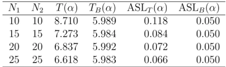
Table 2: Simulated upper percentiles and ASLs of T and TB for (p, d) = (4,1) and α = 0.05 (χ2f(α) = 5.991).
N1 N2 T(α) TB(α) ASLT(α) ASLB(α) 10 10 8.710 5.989 0.118 0.050 15 15 7.273 5.984 0.084 0.050 20 20 6.837 5.992 0.072 0.050 25 25 6.618 5.983 0.066 0.050
Table 3: Simulated upper percentiles and ASLs of T and TB for (p, d) = (4,1) and α = 0.01 (χ2f(α) = 9.210).
N1 N2 T(α) TB(α) ASLT(α) ASLB(α) 10 10 14.996 9.203 0.043 0.010 15 15 11.480 9.196 0.023 0.010 20 20 10.571 9.182 0.018 0.010 25 25 10.199 9.183 0.016 0.010
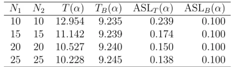
Table 4: Simulated upper percentiles and ASLs of T and TB for (p, d) = (4,2) and α = 0.1 (χ2f(α) = 9.236).
N1 N2 T(α) TB(α) ASLT(α) ASLB(α) 10 10 12.954 9.235 0.239 0.100 15 15 11.142 9.239 0.174 0.100 20 20 10.527 9.240 0.150 0.100 25 25 10.228 9.245 0.138 0.100
Table 5: Simulated upper percentiles and ASLs of T and TB for (p, d) = (4,2) and α = 0.05 (χ2f(α) = 11.071).
N1 N2 T(α) TB(α) ASLT(α) ASLB(α) 10 10 15.947 11.085 0.156 0.050 15 15 13.434 11.086 0.102 0.050 20 20 12.647 11.075 0.084 0.050 25 25 12.267 11.078 0.075 0.050
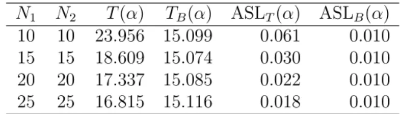
Table 6: Simulated upper percentiles and ASLs of T and TB for (p, d) = (4,2) and α = 0.01 (χ2f(α) = 15.086).
N1 N2 T(α) TB(α) ASLT(α) ASLB(α) 10 10 23.956 15.099 0.061 0.010 15 15 18.609 15.074 0.030 0.010 20 20 17.337 15.085 0.022 0.010 25 25 16.815 15.116 0.018 0.010
Table 7: Simulated upper percentiles and ASLs of T and TB for (p, d) = (4,3) and α = 0.1 (χ2f(α) = 14.684).
N1 N2 T(α) TB(α) ASLT(α) ASLB(α) 10 10 20.662 14.811 0.301 0.104 15 15 17.913 14.747 0.209 0.102 20 20 16.906 14.713 0.173 0.101 25 25 16.358 14.679 0.154 0.100